`merchant-nemhauser` — Merchant & Nemhauser’s (1978) exit-function SO-DTA¶

What. merchant-nemhauser is the first network dynamic traffic assignment model: a discrete-time, single-destination system-optimal program that routes a time-varying demand through links whose outflow is governed by per-link exit functions e_a(t) <= g_a(x_a(t)). This benchmark ships the Carey (1987) LP relaxation (exit as an inequality, not the original nonconvex equality), solved to global optimality by scipy.optimize.linprog (HiGHS).

Why it is in the benchmark. It founds the field of network DTA — every later analytical-DTA model in this track (vi-due, pm-td, lp-so-dta) answers a question this paper first posed. Its distinctive result is that holding traffic back below its exit-function bound (ramp metering) can be STRICTLY optimal, which this notebook demonstrates on a second anchor. See the model compendium (Merchant & Nemhauser 1978) and docs/design/adr-020-merchant-nemhauser.md (P1).

Scope. This notebook solves the LP on two built-in anchors and certifies both; it does not benchmark DTA formulations against each other — for the spillback-capable LP, see lp-so-dta.

Canon. [merchant1978model], [merchant1978optimality], docs/REFERENCES.md / docs/references.bib.

How this notebook is graded¶

A notebook never claims a number it does not compute in that cell. Every scored quantity below is recomputed live by the P1 SODTAEvaluator from the emitted inflow/exit/occupancy arrays alone — conservation, node balance, the exit-function bound, and a weak-duality backstop against the harness’s own freshly-solved LP optimum Z*. The solver’s self-reported objective is never trusted (README, Certified, not self-reported).

# Setup. `merchant-nemhauser` is a core model: a plain `pip install -e .`
# suffices — no optional extra, so no guard cell. The inline backend is
# Agg-based (headless CI renders into the notebook); NEVER
# matplotlib.use("Agg") in-kernel — it silently suppresses inline capture.
%matplotlib inline
import numpy as np

from tabench import (
    SODTAEvaluator,
    mn_metering_scenario,
    mn_parallel_scenario,
    solve_so_dta,
)

Anchor A: parallel-route capacity metering¶

6 vehicles at node 0 choose between a fast capacitated route (g = min(x, 2), 1 period free-flow) and a slow uncapacitated one (2 periods). SODTAScenario is frozen and content-hashed (P2).

scenario_a = mn_parallel_scenario()
print(f"scenario      : {scenario_a.name}")
print(f"content hash  : {scenario_a.content_hash()[:16]}…")
print(f"links={scenario_a.n_links}  nodes={scenario_a.n_nodes}  "
      f"periods={scenario_a.n_periods}  destination={scenario_a.destination}")
print(f"demand at node 0, period 0 : {scenario_a.demand[0, 0]}")

scenario      : mn-parallel
content hash  : 9bbd85f7fd84617f…
links=3  nodes=3  periods=5  destination=2
demand at node 0, period 0 : 6.0

Solve (Anchor A)¶

No Budget/RngBundle/Trace — solve_so_dta builds the canonical LP (canonical_lp) and solves it to global optimality with HiGHS, emitting a DTATrajectory (per-period inflow/exit/occupancy arrays, the P1-certifiable artifact) plus an LP dual certificate.

trajectory_a = solve_so_dta(scenario_a)
print(f"self-reported objective : {trajectory_a.provenance['objective']:.4f}  (provenance only)")
print(f"exits (fast, slow)      : {trajectory_a.exits.round(3).tolist()}")

self-reported objective : 10.0000  (provenance only)
exits (fast, slow)      : [[-0.0, -0.0, 0.0], [2.0, 2.0, -0.0], [2.0, 0.0, 2.0], [0.0, 0.0, -0.0], [-0.0, -0.0, -0.0]]

Certify (P1) — global optimum, via LP duality¶

SODTAEvaluator independently RE-SOLVES the canonical LP at construction (its own fresh Z*), recomputes conservation/node-balance/exit-bound feasibility from the emitted arrays, and verifies the trajectory’s own dual certificate by pure arithmetic (weak duality + zero gap = global optimality) — never trusting either the solver’s claim or its dual.

evaluator_a = SODTAEvaluator(scenario_a)
metrics_a = evaluator_a.certify(trajectory_a)
print(f"feasible            : {metrics_a['feasible']:.0f}")
print(f"so_optimality_gap    : {metrics_a['so_optimality_gap']:.3e}")
print(f"total_cost           : {metrics_a['total_cost']:.4f}")
print(f"dual_gap             : {metrics_a['dual_gap']:.3e}")
print(f"dual_infeasibility   : {metrics_a['dual_infeasibility']:.3e}")
assert metrics_a["feasible"] == 1.0
assert metrics_a["so_optimality_gap"] < 1e-6
assert np.isclose(metrics_a["total_cost"], 10.0, atol=1e-6)
assert metrics_a["dual_gap"] < 1e-6
assert metrics_a["dual_infeasibility"] < 1e-6

feasible            : 1
so_optimality_gap    : 0.000e+00
total_cost           : 10.0000
dual_gap             : 0.000e+00
dual_infeasibility   : 0.000e+00

Anchor B: the strict-holding result¶

A series bottleneck 0 -A-> 1 -B-> 2 where the downstream street is twice as costly per vehicle-period (weight 2 vs 1). The distinctive Merchant- Nemhauser result: the RELAXED (Carey) LP optimum strictly PREFERS holding traffic back on link A below its exit-function bound — metering it at rate 1 while g_A(x_A(1)) = 2 — over the naive equality form e = g(x), which is decision-free here and costs strictly more.

scenario_b = mn_metering_scenario()
trajectory_b = solve_so_dta(scenario_b)
evaluator_b = SODTAEvaluator(scenario_b)
metrics_b = evaluator_b.certify(trajectory_b)
print(f"feasible             : {metrics_b['feasible']:.0f}")
print(f"so_optimality_gap     : {metrics_b['so_optimality_gap']:.3e}")
print(f"total_cost (relaxed)  : {metrics_b['total_cost']:.4f}")
print(f"exit_slack_max        : {metrics_b['exit_slack_max']:.4f}  "
      f"(> 0 means SOME period held traffic below its exit bound)")
assert metrics_b["feasible"] == 1.0
assert metrics_b["so_optimality_gap"] < 1e-6
assert np.isclose(metrics_b["total_cost"], 18.0, atol=1e-6)
# The distinctive result: holding is used (exit bound not tight everywhere).
assert metrics_b["exit_slack_max"] > 0.5
print(f"link A exits (rate-1 metered) : {trajectory_b.exits[:, 0].round(3).tolist()}")

# Recompute the naive equality-form cost DIRECTLY from the scenario's exit
# functions (never quoted): forcing e_a(t) = g_a(x_a(t)) exactly (no holding)
# on this instance is decision-free -- one feasible trajectory -- and it costs
# strictly more than the relaxed optimum.
occ, cost = np.zeros(2), 0.0
x = np.array([0.0, 0.0])
demand = scenario_b.demand[:, 0]
for t in range(scenario_b.n_periods):
    g_a = min(x[0], 2.0)   # exit function g_A(x) = min(x, 2)
    g_b = min(x[1], 1.0)   # exit function g_B(x) = min(x, 1)
    x_next_a = x[0] + demand[t] - g_a
    x_next_b = x[1] + g_a - g_b
    cost += scenario_b.cost_weights[0] * x[0] + scenario_b.cost_weights[1] * x[1]
    x = np.array([x_next_a, x_next_b])
print(f"naive equality-form cost (no holding, recomputed) : {cost:.4f}")
assert cost > metrics_b["total_cost"] + 1.0  # strictly worse than the relaxed optimum

feasible             : 1
so_optimality_gap     : 0.000e+00
total_cost (relaxed)  : 18.0000
exit_slack_max        : 1.0000  (> 0 means SOME period held traffic below its exit bound)
link A exits (rate-1 metered) : [-0.0, 1.0, 1.0, 1.0, 1.0, -0.0, -0.0]
naive equality-form cost (no holding, recomputed) : 22.0000

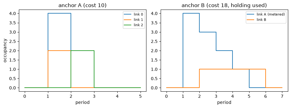
Visualize¶

tabench.viz is a road-network flow visualizer; the M-N artifact is a per-link OCCUPANCY trajectory over discrete periods, not a static link-flow vector, so this notebook plots the certified occupancy trajectories directly (a house time-series plot, not tabench.viz).

import matplotlib.pyplot as plt

fig, axes = plt.subplots(1, 2, figsize=(9.5, 3.6))
for a in range(scenario_a.n_links):
    axes[0].step(range(trajectory_a.occupancies.shape[0]), trajectory_a.occupancies[:, a],
                 where="post", label=f"link {a}")
axes[0].set_title(f"anchor A (cost {metrics_a['total_cost']:.0f})")
axes[0].set_xlabel("period")
axes[0].set_ylabel("occupancy")
axes[0].legend(fontsize=8)

for a, label in enumerate(["A (metered)", "B"]):
    axes[1].step(range(trajectory_b.occupancies.shape[0]), trajectory_b.occupancies[:, a],
                 where="post", label=f"link {label}")
axes[1].set_title(f"anchor B (cost {metrics_b['total_cost']:.0f}, holding used)")
axes[1].set_xlabel("period")
axes[1].legend(fontsize=8)
fig.tight_layout()
display(fig)
plt.close(fig)

../../_images/05a324d13e4e75a1ee6fdb8eb7cd0b4e8285626c70368674cadd874a10bdc7d7.png

Takeaways & pointers¶

Certified, not self-reported. Both anchors’ costs came from SODTAEvaluator, which re-solves the LP itself and cross-checks the dual certificate by pure arithmetic — never the solver’s own objective claim.
Holding is a real phenomenon, not an LP artifact to explain away: anchor B strictly prefers it, at a real cost gap versus the naive exit-equality policy recomputed above.
Where next. the spillback-capable cell LP lp-so-dta (finite storage, which exit functions cannot represent); the lineage in the model compendium.

merchant-nemhauser — Merchant & Nemhauser’s (1978) exit-function SO-DTA¶