sue-msa — Logit stochastic user equilibrium by MSA on the two-route network

What. Stochastic user equilibrium (SUE) replaces Wardrop’s every used route is shortest with every traveller minimises PERCEIVED cost: route choice is a logit model over the true costs, so flow spreads across routes by a dispersion parameter θ. sue-msa reaches the logit-SUE fixed point with the predetermined 1/k successive-averages step over Dial’s efficient-path STOCH loading — no path enumeration ([sheffi1985urban], docs/REFERENCES.md).

Why it is in the benchmark. It is the deterministic-UE ladder’s stochastic counterpart and the anchor for the SUE task (ADR-001). See the model compendium and docs/ARCHITECTURE.md (P1).

Scope. Runs on the built-in two-route logit-SUE anchor (θ = 0.5, demand 4) and certifies the SUE fixed-point residual. It does not treat probit SUE — see sue-probit-msa.

How this notebook is graded

A notebook never claims a number it does not compute in that cell. Every scored quantity below is recomputed live by the P1 Evaluator from the flows the model emitted, in the cell where it is claimed. Model self-reports are shown only as provenance and diffed against the certificate as an honesty check, exactly as the harness treats them (README, Certified, not self-reported).

# Setup. `sue-msa` is a core model: a plain `pip install -e .` suffices — no
# optional extra, so no guard cell. The inline backend is Agg-based (headless CI
# renders into the notebook); NEVER matplotlib.use("Agg") in-kernel — it silently
# suppresses inline figure capture.
%matplotlib inline
import numpy as np

from tabench import (
    Budget,
    DialSUEModel,
    Evaluator,
    RngBundle,
    Trace,
    two_route_scenario,
    viz,
)

The scenario

Two disjoint 2-link routes — A = 1→3→2 (cost 2 + f_A) and B = 1→4→2 (cost 1.5 + 2 f_B) — with demand 4 and logit dispersion θ = 0.5, the analytic logit-SUE anchor. Scenarios are frozen and content-hashed (P2); the hash is the instance’s identity.

scenario = two_route_scenario()
net = scenario.network

print(f"scenario      : {scenario.name}")
print(f"content hash  : {scenario.content_hash()[:16]}…")
print(f"routes        : 1->3->2 (A) and 1->4->2 (B), disjoint")
print(f"total demand  : {scenario.demand.total}")
print(f"SUE family    : {scenario.sue_family} (theta = {scenario.sue_theta})")

scenario      : tworoute
content hash  : 9b98e58b339b702f…
routes        : 1->3->2 (A) and 1->4->2 (B), disjoint
total demand  : 4.0
SUE family    : logit (theta = 0.5)

Solve

The model contract (CONTRIBUTING.md): a model receives (scenario, budget, rng, trace), records checkpoints, and respects the budget. Budgets are hardware-free (iterations / shortest-path calls; wall-clock is recorded but never the ranking axis, P7). Whatever the model writes into self_report is provenance, not a score.

model = DialSUEModel()
bundle = model.solve(scenario, Budget(iterations=300), RngBundle(0), Trace())

final = bundle.final
print(f"model              : {model.name}")
print(f"budget spent       : {final.coords.iterations} iterations, "
      f"{final.coords.sp_calls} shortest-path calls")
print(f"emitted flows      : {np.round(final.link_flows, 6)}")
print(f"self-reported resid: {final.self_report['sue_fixed_point_residual']:.3e}  (provenance only)")

model              : sue-msa
budget spent       : 300 iterations, 301 shortest-path calls
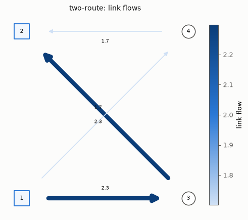
emitted flows      : [2.299096 2.299096 1.700904 1.700904]
self-reported resid: 3.990e-07  (provenance only)

Certify (P1)

The scored quantity for an SUE task is the fixed-point residual — how far the loaded flows are from reproducing themselves under the logit loading — recomputed by the harness Evaluator. The logit loading is closed-form, so the model’s self-report should match the certificate exactly. We recompute the analytic fixed point in-cell with brentq rather than quoting it.

from scipy.optimize import brentq

evaluator = Evaluator(scenario)
metrics = evaluator.evaluate(final.link_flows)
residual = metrics["sue_fixed_point_residual"]
print(f"certified SUE residual : {residual:.3e}")
print(f"feasible               : {metrics['feasible']:.0f}")

assert metrics["feasible"] == 1.0
assert residual < 1e-4

# Honesty diff (P1): the logit loading is closed-form, so self-report == certificate.
assert np.isclose(final.self_report["sue_fixed_point_residual"], residual, rtol=1e-6, atol=1e-12)

# Analytic anchor RECOMPUTED in-cell: the binary-logit fixed point via brentq.
# Route costs c_A = 2 + f_A, c_B = 1.5 + 2 f_B; f_A = D / (1 + exp(theta (c_A - c_B))).
demand = scenario.demand.total
theta = scenario.sue_theta

def _logit_residual(f_a):
    c_a = 2.0 + f_a
    c_b = 1.5 + 2.0 * (demand - f_a)
    return f_a - demand / (1.0 + np.exp(theta * (c_a - c_b)))

f_a = brentq(_logit_residual, 1e-9, demand - 1e-9)
ref_flows = np.array([f_a, f_a, demand - f_a, demand - f_a])
print(f"logit fixed point f_A  : {f_a:.6f}  (recomputed via brentq)")
assert np.allclose(final.link_flows, ref_flows, atol=1e-3)

certified SUE residual : 3.990e-07
feasible               : 1
logit fixed point f_A  : 2.299096  (recomputed via brentq)

Visualize

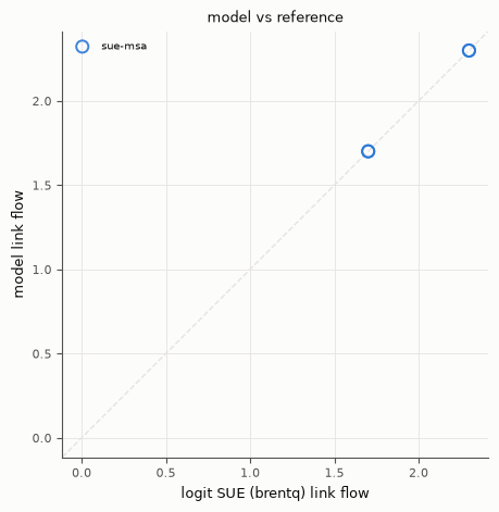
Both figures come from tabench.viz. Left/top: the SUE link flows on the two-route network — flow spreads across BOTH routes (the stochastic spreading θ controls). Right/bottom: the emitted flows against the brentq-recomputed logit fixed point; on-diagonal means the MSA loading reached the analytic SUE.

display(viz.plot_network_flows(net, final.link_flows))
display(viz.plot_flow_scatter(("logit SUE (brentq)", ref_flows), {"sue-msa": final.link_flows}))

Takeaways & pointers

• Certified, not self-reported. The SUE residual came from Evaluator; the closed-form logit self-report was only diffed against it.

• Stochastic spreading. Unlike a deterministic UE, flow uses both routes by the logit dispersion θ — the fixed point recomputed here via brentq.

• Where next. The Monte-Carlo probit variant: sue-probit-msa; the deterministic-UE baseline it mirrors: msa; the ADR-001 SUE design in the model compendium.