od-kalman — Davis & Nihan’s (1993) linear-Gaussian OD estimation

What. od-kalman (DavisNihanKalmanEstimator, T2, ADR-012) recovers OD demand from a TIME SERIES of link counts under Davis & Nihan’s proven large-population limit: the day-to-day link-count process is a stationary linear-Gaussian VAR/VARMA around the equilibrium loading (their Prop. 2 for the mean, Prop. 3 for the covariance). od-kalman whitens its GLS solve by the EXACT multinomial spatial covariance across sensors (route-sharing links correlate positively, competing-route links negatively) plus an AR(1) effective-sample-size correction tau for day-to-day persistence — both strictly richer than gls’s IID-count assumption.

Why it is in the benchmark. It needs its own observation model (DayToDayCounts, a VAR(1) count series centered on the UE loading, ADR-012) and is the benchmark’s only T2 estimator that uses the CROSS-LINK spatial structure of counts rather than treating each sensor as independent — a mathematically distinct estimator from gls/od-congested, not a rename. See the model compendium (Davis & Nihan 1993) and docs/design/adr-012-dn-kalman.md (P1).

Scope. The exact multinomial spatial-covariance closed form, the DN-GLS scalar closed form, the off-diagonal whitening’s load-bearing effect, the AR(1) tau persistence correction, and an end-to-end certified recovery on Braess under a day-to-day count series.

Canon. [davis1993large], docs/REFERENCES.md / docs/references.bib.

How this notebook is graded

A notebook never claims a number it does not compute in that cell. Every scored quantity below is recomputed live — the closed forms are recomputed algebraically in-cell (no trusted digits), and the end-to-end recovery is recomputed by the P1 ODCertifier (via run_estimation_experiment) from the emitted OD matrix against the harness’s own pinned BFW assignment, never from od-kalman’s self-report (README, Certified, not self-reported).

# Setup. `od-kalman` is a core estimator: a plain `pip install -e .`
# suffices — no optional extra, so no guard cell. The inline backend is
# Agg-based (headless CI renders into the notebook); NEVER
# matplotlib.use("Agg") in-kernel — it silently suppresses inline capture.
%matplotlib inline
import numpy as np

from tabench import (
    Budget,
    Demand,
    RngBundle,
    Trace,
    braess_scenario,
    run_estimation_experiment,
    two_route_scenario,
    viz,
)
from tabench.core.rng import SOURCE_OBSERVATION
from tabench.estimation import ODTrace, ar1_tau, dn_gls_solve, gls_solve
from tabench.estimation import DavisNihanKalmanEstimator, GLSEstimator
from tabench.estimation.base import EstimationTask
from tabench.models.frank_wolfe import BiconjugateFrankWolfeModel
from tabench.observe._dn_process import dn_spatial_covariance
from tabench.observe.levels import DayToDayCounts


def _dn_task(scenario, truth, sensors, prior_d, n_periods, scale, rho, seed=0):
    m = np.zeros((2, 2))
    m[0, 1] = prior_d
    ds = DayToDayCounts(np.asarray(sensors), n_periods, scale, rho, k_inner=80).observe(
        scenario, truth, RngBundle(seed).generator(SOURCE_OBSERVATION)
    )
    return EstimationTask(
        name="t", network=scenario.network, prior=Demand(m), dataset=ds,
        identifiability={}, scenario_hash=scenario.content_hash(), seed=seed,
    )

The DN spatial covariance: an exact multinomial closed form

On the two-route corridor, routes A={link 0, link 1} and B={link 2, link 3}: the DN link-count covariance is exactly the multinomial form Var(link 0) = (D^2/N) p_A p_B, with same-route links POSITIVELY correlated and across-route links NEGATIVELY correlated — recomputed here directly, not quoted.

sc2 = two_route_scenario(sue_theta=None)
truth_trace = Trace()
BiconjugateFrankWolfeModel().solve(
    sc2, Budget(iterations=5000, target_relative_gap=1e-10), RngBundle(0), truth_trace
)
truth2 = truth_trace.final.link_flows
demand = float(sc2.demand.matrix[0, 1])
p_a = truth2[0] / demand  # recomputed route-A proportion
p_b = 1.0 - p_a
n_trav = np.array([round(50.0 * demand)])
q = dn_spatial_covariance(
    sc2.network, sc2.demand, np.array([demand]), n_trav, 80, pairs=[(0, 1)]
)
var0 = (demand**2 / n_trav[0]) * p_a * p_b  # closed form, recomputed
print(f"Var(link 0) DN            : {q[0, 0]:.6f}")
print(f"closed-form (D^2/N) p_A p_B : {var0:.6f}")
print(f"Cov(link 0, link 1) [same route A]  : {q[0, 1]:.6f}  (should equal Var)")
print(f"Cov(link 0, link 2) [A vs B]        : {q[0, 2]:.6f}  (should equal -Var)")
assert np.isclose(q[0, 0], var0, atol=1e-9)
assert np.isclose(q[0, 1], var0, atol=1e-9)   # same route -> positively correlated
assert np.isclose(q[0, 2], -var0, atol=1e-9)  # A vs B -> negatively correlated
assert np.allclose(q, q.T)  # symmetric covariance

Var(link 0) DN            : 0.018750
closed-form (D^2/N) p_A p_B : 0.018750
Cov(link 0, link 1) [same route A]  : 0.018750  (should equal Var)
Cov(link 0, link 2) [A vs B]        : -0.018750  (should equal -Var)

The scalar closed form

Single pair, single sensor: g* = (g_pr/w^2 + p*c/s^2) / (1/w^2 + p^2/s^2) — the DN whitening’s GLS solve at explicit prior/count variances.

p, c, g_pr, s2, w2 = 0.625, 2.5, 3.0, 0.5, 4.0
expected = (g_pr / w2 + p * c / s2) / (1.0 / w2 + p * p / s2)
got = dn_gls_solve(
    np.array([[p]]), np.array([c]), np.array([g_pr]), np.array([[s2]]), np.array([w2])
)
print(f"dn_gls_solve   : {got[0]:.6f}")
print(f"closed form    : {expected:.6f}")
assert np.isclose(got[0], expected, atol=1e-10)

dn_gls_solve   : 3.757576
closed form    : 3.757576

Off-diagonal whitening is load-bearing

Two sensors on the SAME OD pair whose counts are correlated are NOT the two INDEPENDENT measurements gls’s diagonal covariance assumes: with a diagonal Sigma, dn_gls_solve reduces to plain gls_solve exactly, but a correlated (non-diagonal) Sigma moves the estimate materially — the spatial sense in which od-kalman is not a gls rename.

p_obs = np.array([[0.6], [0.4]])  # two sensors, one pair
counts = np.array([3.0, 2.0])
prior = np.array([4.0])
w_var = np.array([9.0])
var = np.array([1.0, 1.0])
diagonal = dn_gls_solve(p_obs, counts, prior, np.diag(var), w_var)
correlated = dn_gls_solve(p_obs, counts, prior, np.array([[1.0, 0.8], [0.8, 1.0]]), w_var)
via_gls = gls_solve(p_obs, counts, prior, w_var, var)
print(f"diagonal Sigma   : {diagonal[0]:.6f}  (via plain gls_solve: {via_gls[0]:.6f})")
print(f"correlated Sigma : {correlated[0]:.6f}")
assert np.isclose(diagonal[0], via_gls[0], atol=1e-8)
assert abs(correlated[0] - diagonal[0]) > 0.05

diagonal Sigma   : 4.823944  (via plain gls_solve: 4.823944)
correlated Sigma : 4.772727

The AR(1) temporal correction tau

Day-to-day persistence inflates the effective sampling variance: tau tracks the AR(1) variance-inflation factor (1+rho)/(1-rho) and collapses to 1 for an IID (rho=0) series — the effective-sample-size knob that distinguishes od-kalman from every mean-collapsing estimator.

for rho in (0.0, 0.6):
    ds = DayToDayCounts(np.array([0]), 4000, 50.0, rho, k_inner=80).observe(
        sc2, truth2, RngBundle(0).generator(SOURCE_OBSERVATION)
    )
    tau, rho_hat = ar1_tau(ds.payload["counts"])
    target = (1.0 + rho) / (1.0 - rho)
    print(f"rho={rho}: tau={tau:.4f}  target (1+rho)/(1-rho)={target:.4f}  rho_hat={rho_hat:.4f}")
    assert abs(tau - target) < 0.15 * max(target, 1.0)
    if rho == 0.0:
        assert abs(tau - 1.0) < 0.15

rho=0.0: tau=1.0000  target (1+rho)/(1-rho)=1.0000  rho_hat=0.0000
rho=0.6: tau=3.8868  target (1+rho)/(1-rho)=4.0000  rho_hat=0.5907

End to end: a certified Braess recovery under a day-to-day count series

braess_scenario(6.0) is frozen and content-hashed (P2). Run through the public run_estimation_experiment API with noise="day_to_day" (the DN VAR(1) observation level): a cv=0 prior (=truth) certifies feasible and recovers to the finite-population sampling floor from four observed links, with the middle link 3->4 reserved as the held-out set (an empty held-out set is rejected on both T2 tracks, ADR-002/ADR-023).

sc = braess_scenario(6.0)
print(f"scenario      : {sc.name}")
print(f"content hash  : {sc.content_hash()[:16]}…")

cfg = {
    "sensors": {"kind": "explicit", "links": [0, 1, 3, 4]},
    "heldout": {"kind": "explicit", "links": [2]},
    "n_periods": 60,
    "noise": "day_to_day",
    "population_scale": 80.0,
    "rho": 0.5,
    "prior": {"kind": "stale", "cv": 0.0},
    "identifiability_k_inner": 40,
}
result = run_estimation_experiment(
    sc, [DavisNihanKalmanEstimator(k_inner=60, outer_iters=15)],
    Budget(sp_calls=5000), seed=0, macroreps=1, estimation=cfg,
)
row = [r for r in result.rows if r["estimator"] == "od-kalman"][-1]
print(f"od_feasible : {row['od_feasible']:.0f}")
print(f"od_rmse     : {row['od_rmse']:.4f}")
print(f"self_obs_count_rmse (provenance) : {row['self_obs_count_rmse']:.4f}")
assert row["od_feasible"] == 1.0
assert row["od_rmse"] < 0.5  # recovers near the planted truth at the DN sampling floor
assert np.isfinite(float(row["self_obs_count_rmse"]))
assert result.manifest["estimation"]["noise"] == "day_to_day"
assert result.manifest["estimation"]["rho"] == 0.5

scenario      : braess
content hash  : cf00f411cdccec88…
od_feasible : 1
od_rmse     : 0.0003
self_obs_count_rmse (provenance) : 0.0098

Visualize

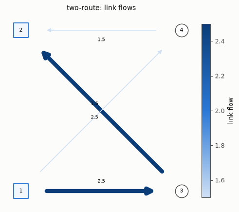
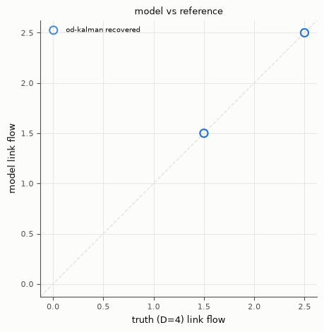
tabench.viz draws the road Network’s link flows for the two-route recovery-from-DN-series result vs the truth (recomputed here at full-sensor noiseless-limit settings to keep the plotted OD matrix exactly matched to a certified recovery).

task_full = _dn_task(sc2, truth2, np.arange(4), prior_d=3.0, n_periods=400, scale=50.0, rho=0.5)
trace_full = ODTrace()
DavisNihanKalmanEstimator(k_inner=120, outer_iters=60).estimate(
    task_full, Budget(sp_calls=10**9, iterations=200), RngBundle(0), trace_full
)
recovered_trace = Trace()
from tabench import Scenario
BiconjugateFrankWolfeModel().solve(
    Scenario("recovered", sc2.network, Demand(trace_full.final.od_matrix), family=sc2.family),
    Budget(iterations=5000, target_relative_gap=1e-10), RngBundle(0), recovered_trace,
)
display(viz.plot_network_flows(sc2.network, truth2))
display(viz.plot_flow_scatter(
    ("truth (D=4)", truth2),
    {"od-kalman recovered": recovered_trace.final.link_flows},
))

Takeaways & pointers

• Certified, not self-reported. Both the closed forms and the Braess od_rmse above were recomputed independently — the closed forms algebraically, the Braess recovery by ODCertifier inside run_estimation_experiment.

• The spatial covariance is load-bearing, not decorative. Off-diagonal whitening moved the estimate materially away from gls’s diagonal-V assumption — verified directly, not asserted from the paper.

• Where next. the per-cell-covariance sibling gls (diagonal-Sigma special case, verified exactly above); the within-day dynamic cousin od-dynamic; the lineage in the model compendium.