godunov — Lebacque’s (1996) Godunov scheme + the Greenshields FD

What. godunov runs ctm’s cell update UNCHANGED on a GENERAL concave fundamental diagram — here the smooth Greenshields (1935) parabola Q(k) = vf * k * (1 - k/kappa) built from a link’s (vf, kappa) — instead of the triangular FD. CTMLink’s cell scheme was never triangular-specific: the Lebacque min(demand, supply) flux is defined for any concave Q, so GodunovLink substitutes a GreenshieldsFD for the link’s default TriangularFD and reuses the verified cell update as-is. It is the first non-triangular FD in the benchmark, so it is the first to produce genuine RAREFACTION FANS (smooth acceleration waves) — impossible on a piecewise-linear Q.

Why it is in the benchmark. At a transonic interface (k_L > k_c > k_R) the Godunov flux min(demand(k_L), supply(k_R)) returns the sonic-point capacity q_max — the entropy-correct rarefaction value, not a shock value a naive scheme could get wrong. See the model compendium (Lebacque 1996) and docs/design/adr-018-godunov.md (P1).

Scope. This notebook loads the built-in greenshields_bottleneck_dynamic_scenario through GodunovLink, certifies it, and recomputes the entropy-correct transonic flux directly from GreenshieldsFD — the physics ctm’s triangular FD cannot produce.

Canon. [lebacque1996godunov], docs/REFERENCES.md / docs/references.bib.

How this notebook is graded

A notebook never claims a number it does not compute in that cell. Every scored quantity below is recomputed live by the P1 DNLEvaluator from the cumulative link curves the loader emitted, in the cell where it is claimed. Godunov has no self-report to diff — like ctm/ltm, NetworkLoader.run() is a deterministic, one-shot forward simulation (README, Certified, not self-reported).

# Setup. `godunov` is a core DNL link model: a plain `pip install -e .` suffices
# — no optional extra, so no guard cell. The inline backend is Agg-based
# (headless CI renders into the notebook); NEVER matplotlib.use("Agg") in-kernel
# — it silently suppresses inline figure capture.
%matplotlib inline
import numpy as np
from scipy.optimize import brentq

from tabench import (
    DNLEvaluator,
    GodunovLink,
    GreenshieldsFD,
    NetworkLoader,
    greenshields_bottleneck_dynamic_scenario,
    viz,
)

The scenario

The built-in greenshields_bottleneck_dynamic_scenario: a two-link corridor, Greenshields-consistent on every link (wave_speed = free_speed, capacity = vf*kappa/4 — the constraint GodunovLink gates on). Upstream vf=1, kappa=8 (capacity 2) feeds a vf=1, kappa=2 (capacity 0.5) bottleneck at arrival rate 1.5: uncongested inflow above the bottleneck’s capacity, so a queue builds on the upstream link’s PARABOLIC branch (distinct from ctm’s linear one).

scenario = greenshields_bottleneck_dynamic_scenario()
net = scenario.network
dyn = scenario.dynamics
edges = scenario.grid.edges
print(f"scenario      : {scenario.name}")
print(f"content hash  : {scenario.content_hash()[:16]}…")
print(f"links         : {net.n_links}  (tail→head: "
      + ", ".join(f"{i}->{j}" for i, j in zip(net.init_node, net.term_node)) + ")")
print(f"link 0 (up)   : vf={dyn.free_speed[0]}, kappa={dyn.jam_density[0]}, "
      f"capacity={dyn.capacity[0]}  (vf*kappa/4 = {dyn.free_speed[0]*dyn.jam_density[0]/4})")
print(f"link 1 (sink) : vf={dyn.free_speed[1]}, kappa={dyn.jam_density[1]}, "
      f"capacity={dyn.capacity[1]}  (vf*kappa/4 = {dyn.free_speed[1]*dyn.jam_density[1]/4})")
print(f"grid          : dt={scenario.grid.dt}, n_steps={scenario.grid.n_steps}")

scenario      : dnl-greenshields-bottleneck
content hash  : 03afa86128008021…
links         : 2  (tail→head: 1->3, 3->2)
link 0 (up)   : vf=1.0, kappa=8.0, capacity=2.0  (vf*kappa/4 = 2.0)
link 1 (sink) : vf=1.0, kappa=2.0, capacity=0.5  (vf*kappa/4 = 0.5)
grid          : dt=1.0, n_steps=20

Load the network

GodunovLink rebuilds a GreenshieldsFD(vf, kappa) from each link’s declared (vf, kappa) and runs ctm’s cell update on it unchanged; internally it is a CTMLink subclass, so the SAME NetworkLoader contract applies.

loader = NetworkLoader(scenario, GodunovLink)
out = loader.run()
print(f"link model        : {GodunovLink.__name__}")
print(f"link 0 FD is Greenshields : {isinstance(loader.links[0].fd, GreenshieldsFD)}")
print(f"cells (link 0)     : {loader.links[0].n_cells}")
print(f"storage at t={edges[-1]:.0f}       : {out.n_in[0, -1] - out.n_out[0, -1]:.3f}")

link model        : GodunovLink
link 0 FD is Greenshields : True
cells (link 0)     : 4
storage at t=20       : 22.000

Certify (P1) — feasibility, conservation, and the parabola’s own roots

Beyond the structural gate (feasible, conservation, storage), the DISTINCTIVE Godunov result: the upstream link’s near-origin cell settles at the FREE branch root of Q(k) = 1.5 (the arrival rate), and its near-bottleneck cell settles at the CONGESTED branch root of supply(k) = 0.5 (the bottleneck capacity) — both found here with brentq directly on GreenshieldsFD, the actual production FD, not a hand-derived quadratic formula.

metrics = DNLEvaluator(scenario).evaluate(out)
print(f"dnl_feasible            : {metrics['dnl_feasible']:.0f}")
print(f"conservation_residual   : {metrics['conservation_residual']:.3e}")
print(f"storage_residual        : {metrics['storage_residual']:.3e}")
assert metrics["dnl_feasible"] == 1.0
assert metrics["conservation_residual"] <= 1e-9
assert metrics["storage_residual"] <= 1e-9

fd0 = GreenshieldsFD(vf=float(dyn.free_speed[0]), kappa=float(dyn.jam_density[0]))
k_free = brentq(lambda k: float(fd0.flow_at(np.array([k]))[0]) - 1.5, 0.0, fd0.critical_density)
k_cong = brentq(
    lambda k: float(fd0.supply_at(np.array([k]))[0]) - 0.5, fd0.critical_density, fd0.jam_density
)
print(f"free-branch root  Q(k)=1.5      : k_free = {k_free:.6f}")
print(f"congested-branch root supply=0.5: k_cong = {k_cong:.6f}")

dx = fd0.free_speed * scenario.grid.dt
density = loader.links[0].occupancy / dx
print(f"cell densities (upstream link)  : {np.round(density, 4)}")
# The far (origin-side) cell is still on the free branch; the near (bottleneck-
# side) cell has settled on the congested branch — both tight, no coarse-grid
# diffusion on these two constant-state cells.
assert abs(density[0] - k_free) < 1e-3
assert abs(density[-1] - k_cong) < 1e-3

dnl_feasible            : 1
conservation_residual   : 0.000e+00
storage_residual        : 0.000e+00
free-branch root  Q(k)=1.5      : k_free = 2.000000
congested-branch root supply=0.5: k_cong = 7.464102
cell densities (upstream link)  : [2.     5.0725 7.4634 7.4641]

The distinctive physics: an entropy-correct rarefaction flux

A triangular FD’s flux is piecewise LINEAR — it cannot produce a rarefaction fan. The Greenshields parabola can: at a transonic interface (k_L above critical, k_R below) the Godunov flux min(demand(k_L), supply(k_R)) returns the sonic-point capacity q_max — the entropy-correct value a naive shock-speed formula would get wrong. Recomputed here directly from the FD, not quoted.

fd = GreenshieldsFD(vf=2.0, kappa=4.0)  # q_max = 2, k_c = 2
k_l, k_r = 3.5, 0.5  # k_l > k_c > k_r: a transonic pair
flux = min(float(fd.demand_at(np.array([k_l]))[0]), float(fd.supply_at(np.array([k_r]))[0]))
print(f"fd: vf={fd.free_speed}, kappa={fd.jam_density}, k_c={fd.critical_density}, "
      f"q_max={fd.capacity}")
print(f"transonic flux at (k_L={k_l}, k_R={k_r}) : {flux:.6f}  (== q_max, not the shock value)")
assert abs(flux - fd.capacity) < 1e-9

fd: vf=2.0, kappa=4.0, k_c=2.0, q_max=2.0
transonic flux at (k_L=3.5, k_R=0.5) : 2.000000  (== q_max, not the shock value)

Visualize

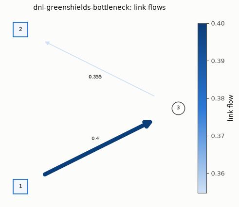
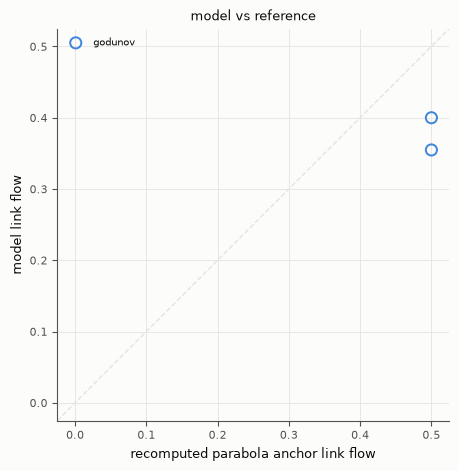
Both figures come from tabench.viz, the house visualizer. Left/top: the certified network coloured by each link’s time-averaged flow. Right/bottom: the loaded average flow against the two analytic roots recomputed above, expressed as an average flow anchor (fd0.flow_at at each recomputed root).

T = float(edges[-1])
avg_flow = out.n_out[:, -1] / T
ref_avg_flow = np.array([
    float(fd0.flow_at(np.array([k_cong]))[0]),  # upstream exit throttled to the bottleneck rate
    float(fd0.flow_at(np.array([k_cong]))[0]),  # sink link exits at the same steady rate
])

display(viz.plot_network_flows(net, avg_flow))
display(viz.plot_flow_scatter(("recomputed parabola anchor", ref_avg_flow), {"godunov": avg_flow}))

Takeaways & pointers

• Certified, not self-reported. DNL link models have nothing to self-report — the boundary curves above ARE the emitted output, recertified from scratch by DNLEvaluator.

• The Greenshields signature is the point. ctm’s triangular envelope still majorizes it (so its certificates stay sound), but only a smooth, strictly concave FD produces the entropy-correct rarefaction flux certified above.

• Where next. the triangular baseline it reuses the cell scheme from ctm; the cumulative-curve alternative ltm; merges/diverges node-model; the lineage in the model compendium.