dtd-unifying — Cantarella & Cascetta’s (1995) unifying day-to-day process

What. One two-equation process — a cost-learning filter p ← (1−w) p + w t(v) plus a choice update where a fraction α reconsiders at forecast costs — whose choice map is gated per scenario (AON best response ⇒ Wardrop UE on deterministic tasks; Dial logit ⇒ logit SUE on SUE tasks). The unifying node of the day-to-day family.

Why it is in the benchmark. It reduces exactly to dtd-horowitz (α=1) and to msa (w=1, α=1), and exhibits the joint (α, w) flip-stability boundary: at (1,1) it limit-cycles while EITHER cost memory OR choice inertia restores convergence (C&C’s headline result). See the model compendium and the certificate design in docs/ARCHITECTURE.md (P1).

Scope. Runs the process on a built-in scenario and certifies the result; it does not benchmark day-to-day models against each other. Reference: Cantarella & Cascetta (1995), Transportation Science 29(4).

Canon. [cantarella1995dynamic], docs/REFERENCES.md / docs/references.bib.

How this notebook is graded

A notebook never claims a number it does not compute in that cell. Every scored quantity below is recomputed live by the P1 Evaluator from the flows the model emitted, in the cell where it is claimed. Model self-reports (the per-day gap/residual, the Lyapunov value) are shown only as provenance and diffed against the certificate, exactly as the harness treats them (README, Certified, not self-reported).

# Setup. `dtd-unifying` is a core day-to-day model: a plain `pip install -e .` suffices —
# no optional extra, so no guard cell. The inline backend is Agg-based (headless CI
# renders into the notebook); NEVER matplotlib.use("Agg") in-kernel — it silently
# suppresses inline figure capture.
%matplotlib inline
import numpy as np

from tabench import (
    Budget,
    CostSmoothingSUEModel,
    Evaluator,
    MSAModel,
    RngBundle,
    Trace,
    UnifyingDTDModel,
    braess_scenario,
    two_route_scenario,
    viz,
)

The scenario

The built-in two-route logit-SUE anchor (demand 4, dispersion θ=0.5): route A cost 2+f_A, route B cost 1.5+2 f_B. Its rest point is the binary-logit stochastic user equilibrium, recomputed analytically in the certify cell — NOT the deterministic Wardrop UE.

scenario = two_route_scenario()
net = scenario.network
print(f"scenario      : {scenario.name}")
print(f"content hash  : {scenario.content_hash()[:16]}…")
print(f"links         : {net.n_links}  (tail→head: "
      + ", ".join(f"{i}->{j}" for i, j in zip(net.init_node, net.term_node)) + ")")
print(f"total demand  : {scenario.demand.total}")
print("task          : logit SUE, θ=0.5")

scenario      : tworoute
content hash  : 9b98e58b339b702f…
links         : 4  (tail→head: 1->3, 3->2, 1->4, 4->2)
total demand  : 4.0
task          : logit SUE, θ=0.5

Run the adjustment process

The model contract (CONTRIBUTING.md): a model receives (scenario, budget, rng, trace) and records one checkpoint per day — here a budget iteration is a day. Everything the model writes into self_report (the per-day gap/residual, the Lyapunov value) is provenance, not a score.

bundle_trace = Trace()
model = UnifyingDTDModel()  # default (memory_weight=0.5, reconsideration_rate=0.5)
# Full horizon so both the SUE residual and the forecast (perceived-cost) gap vanish.
model.solve(scenario, Budget(iterations=500), RngBundle(0), bundle_trace)
final = bundle_trace.final
print(f"model            : {model.name}")
print(f"days simulated   : {final.coords.iterations}  "
      f"({final.coords.sp_calls} shortest-path calls)")
print(f"emitted flows    : {np.round(final.link_flows, 6)}")
print(f"self-reported residual: {final.self_report['sue_fixed_point_residual']:.3e}  (provenance only)")

model            : dtd-unifying
days simulated   : 500  (1001 shortest-path calls)
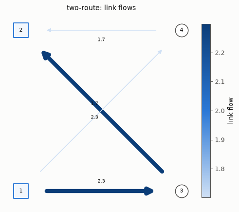
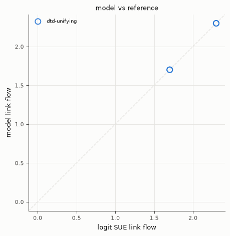
emitted flows    : [2.299096 2.299096 1.700904 1.700904]
self-reported residual: 3.331e-16  (provenance only)

Certify (P1) — the SUE fixed point AND the descent

The harness recomputes the ADR-001 Dial-STOCH residual from the emitted flows. Certified here: (1) the terminal flows are the logit SUE — residual → 0 with the analytic binary- logit anchor recomputed in-cell, while the deterministic UE gap stays positive (a descriptive column, like sue-msa); (2) the model’s Lyapunov / provenance signature.

from scipy.optimize import brentq
evaluator = Evaluator(scenario)
metrics = evaluator.evaluate(final.link_flows)
residual = metrics["sue_fixed_point_residual"]
print(f"certified SUE residual : {residual:.3e}")
print(f"feasible               : {metrics['feasible']:.0f}")
print(f"UE relative gap        : {metrics['relative_gap']:.3f}  (stays >0 — logit SUE ≠ deterministic UE)")
assert metrics["feasible"] == 1.0
assert residual < 1e-6
assert metrics["relative_gap"] > 0.01  # descriptive column: not the deterministic UE

# Analytic binary-logit SUE anchor, recomputed in-cell (θ=0.5, demand 4): the root of
# f_A = D / (1 + exp(θ(c_A − c_B))), c_A = 2 + f_A, c_B = 1.5 + 2(4 − f_A).
def _resid(f_a):
    c_a, c_b = 2.0 + f_a, 1.5 + 2.0 * (4.0 - f_a)
    return f_a - 4.0 / (1.0 + np.exp(0.5 * (c_a - c_b)))
f_a = brentq(_resid, 0.0, 4.0, xtol=1e-12)
ref_flows = np.array([f_a, f_a, 4.0 - f_a, 4.0 - f_a])
print(f"analytic logit SUE f_A : {f_a:.6f}")
assert np.allclose(final.link_flows, ref_flows, atol=1e-4)
# Honesty (P1): the model self-reports the SAME residual the harness recomputes.
assert np.isclose(
    final.self_report["sue_fixed_point_residual"], residual, rtol=1e-9, atol=1e-12
)
# The perceived-cost (forecast) gap vanishes at rest (provenance).
pgap = [s.self_report["perceived_cost_gap"] for s in bundle_trace]
assert max(pgap) > 1.0 and pgap[-1] < 1e-6
print(f"perceived-cost gap     : {max(pgap):.3g} → {pgap[-1]:.2e}")

# DISTINCTIVE (Cantarella & Cascetta 1995): joint (α, w) flip stability. At (α,w)=(1,1)
# — no choice inertia, no cost memory — the process limit-cycles; EITHER form of inertia
# restores convergence. The default (0.5, 0.5) is stable (certified above); the contrast:
cyc = Trace()
UnifyingDTDModel(memory_weight=1.0, reconsideration_rate=1.0).solve(
    scenario, Budget(iterations=400), RngBundle(0), cyc
)
print(f"(α,w)=(1,1) residual   : {cyc.final.self_report['sue_fixed_point_residual']:.3f}  (limit cycle)")
assert cyc.final.self_report["sue_fixed_point_residual"] > 1.0

certified SUE residual : 3.331e-16
feasible               : 1
UE relative gap        : 0.056  (stays >0 — logit SUE ≠ deterministic UE)
analytic logit SUE f_A : 2.299096
perceived-cost gap     : 2.79 → 0.00e+00
(α,w)=(1,1) residual   : 3.323  (limit cycle)

The exact reductions: α=1 → dtd-horowitz, (w=1, α=1) → msa

The docstring’s central claim — this model UNIFIES the previously separate day-to-day strands — is not narrative unless it is checkpoint-exact, and the claim is stronger than “reaches the same fixed point”: it is day-by-day trajectory identity, verified below at rtol=atol=1e-12. reconsideration_rate=1.0 (everyone reconsiders daily) collapses the choice update v <- v + alpha (y - v) to v <- y, which — on the SAME stochastic-branch anchor, at the SAME memory weight w — is dtd-horowitz’s own recursion verbatim; likewise memory_weight=1.0 collapses the cost filter to p <- t(v) (no memory), and at alpha=1 too the deterministic branch’s annealed step alpha/n = 1/n IS msa’s own iterate sequence on the SAME Braess anchor. Both hold up to a one-checkpoint index offset: dtd-unifying updates p at the START of each loop iteration (folding its day-0 bootstrap into day 1’s update), while dtd-horowitz/msa record-then-update at the END of theirs — a loop-boundary bookkeeping difference, not an approximation (RNG plays no role in either process; both are deterministic recursions). Mirrors tests/test_dtd_unifying.py’s test_reduces_to_dtd_horowitz_at_alpha_one / test_reduces_to_msa_at_unit_memory_and_alpha verbatim.

# α=1 → dtd-horowitz, stochastic branch, SAME two-route SUE anchor, SAME w=0.5.
unifying_h = Trace()
UnifyingDTDModel(memory_weight=0.5, reconsideration_rate=1.0).solve(
    scenario, Budget(iterations=30), RngBundle(0), unifying_h
)
horowitz = Trace()
CostSmoothingSUEModel(smoothing_weight=0.5).solve(
    scenario, Budget(iterations=31), RngBundle(0), horowitz
)
# One-day offset: dtd-unifying's checkpoint k is dtd-horowitz's checkpoint k+1.
max_diff_h = max(
    np.abs(unifying_h.checkpoints[k].link_flows - horowitz.checkpoints[k + 1].link_flows).max()
    for k in range(30)
)
print(f"dtd-unifying(α=1) vs dtd-horowitz, max |Δflow| over 30 days : {max_diff_h:.2e}")
for k in range(30):
    np.testing.assert_allclose(
        unifying_h.checkpoints[k].link_flows,
        horowitz.checkpoints[k + 1].link_flows,
        rtol=1e-12, atol=1e-12,
    )

# (w=1, α=1) → msa, deterministic branch, SAME Braess anchor.
braess = braess_scenario()
unifying_m = Trace()
UnifyingDTDModel(memory_weight=1.0, reconsideration_rate=1.0).solve(
    braess, Budget(iterations=40), RngBundle(0), unifying_m
)
msa = Trace()
MSAModel().solve(braess, Budget(iterations=41), RngBundle(0), msa)
max_diff_m = max(
    np.abs(unifying_m.checkpoints[k].link_flows - msa.checkpoints[k + 1].link_flows).max()
    for k in range(40)
)
print(f"dtd-unifying(w=1,α=1) vs msa, max |Δflow| over 40 days      : {max_diff_m:.2e}")
for k in range(40):
    np.testing.assert_allclose(
        unifying_m.checkpoints[k].link_flows,
        msa.checkpoints[k + 1].link_flows,
        rtol=1e-12, atol=1e-12,
    )

dtd-unifying(α=1) vs dtd-horowitz, max |Δflow| over 30 days : 0.00e+00
dtd-unifying(w=1,α=1) vs msa, max |Δflow| over 40 days      : 0.00e+00

Visualize

Both figures come from tabench.viz, the house visualizer — every plotted number is one certified above. Left/top: the certified terminal link flows on the network. Right/bottom: the emitted flows against the fixed point recomputed in the certify cell — points on the y = x guide mean the day-to-day process settled on it link-for-link.

# Certified terminal flows on the network (house style via tabench.viz).
display(viz.plot_network_flows(net, final.link_flows))

# Emitted flows vs the logit SUE recomputed above (off-diagonal == not settled).
display(viz.plot_flow_scatter(("logit SUE", ref_flows), {"dtd-unifying": final.link_flows}))

Takeaways & pointers

• Certified, not self-reported. The residual came from Evaluator; the contrast run at (α,w)=(1,1) certified an O(1) limit cycle — either form of inertia is what makes the default converge.

• The day-to-day signature is the point. A UE/SUE solver gives you the fixed point; a day-to-day model gives you the adjustment path to it.

• Both exact reductions are certified above, checkpoint-by-checkpoint (not just at the terminal flow): dtd-horowitz (α=1) and msa (w=α=1). The stochastic process dtd-stochastic is the OTHER generalization axis (a genuinely stochastic process, vs this model’s deterministic recursion over a probabilistic choice map).

• Where next. the lineage in the model compendium.