od-dynamic — Cascetta, Inaudi & Marquis’s (1993) within-day dynamic OD estimation
What. od-dynamic (T2d, ADR-023) estimates a SEQUENCE of time-sliced OD
matrices d_h from time-sliced link counts, linked by an EXOGENOUS lagged
assignment map (frozen free-flow travel times — no iterative equilibrium).
The paper offers two GLS variants: SIMULTANEOUS (all slices jointly,
efficient but needs the whole horizon before solving) and SEQUENTIAL (slice
by slice, earlier estimates frozen once made — online-capable, but provably
less efficient). This notebook covers all three registered T2d units:
od-dynamic-sim, od-dynamic-seq, and the prior-profile baseline they
must both beat.
Why it is in the benchmark. It is the benchmark’s first WITHIN-DAY
estimation task — the estimand is a (H, Z, Z) demand PROFILE, not a single
(Z, Z) matrix, and the exogenous lag tensor is a genuinely new artifact
(no assignment equilibrium is solved; certification is exact linear
algebra). The simultaneous/sequential efficiency gap is the paper’s
headline result, made an executable, hand-verified fact below. See the
model compendium (Cascetta, Inaudi & Marquis 1993)
and
docs/design/adr-023-od-dynamic.md
(P1).
Scope. Anchor A1 (integer lag: both estimators reduce EXACTLY to the
static gls closed form, per slice); Anchor A2 (fractional lag — “the”
anchor: simultaneous strictly dominates sequential, exact rationals); and an
end-to-end certified run on the two-route corridor via the public
run_dynamic_estimation_experiment API.
Canon. [cascetta1993dynamic], docs/REFERENCES.md / docs/references.bib.
How this notebook is graded
A notebook never claims a number it does not compute in that cell. Every
scored quantity below is recomputed live — the anchors are recomputed as
exact closed forms in-cell (no trusted digits, exact rationals via
fractions.Fraction where the paper’s own algebra is being verified), and
the end-to-end recovery is recomputed by the P1 DynamicODCertifier (via
run_dynamic_estimation_experiment) from the emitted OD profile, never from
the estimator’s self-report
(README, Certified, not self-reported).
# Setup. `od-dynamic` is a core estimator family: a plain `pip install -e .`
# suffices — no optional extra, so no guard cell. The inline backend is
# Agg-based (headless CI renders into the notebook); NEVER
# matplotlib.use("Agg") in-kernel — it silently suppresses inline capture.
%matplotlib inline
from fractions import Fraction

import numpy as np

from tabench import (
    Budget,
    DynamicPriorBaseline,
    RngBundle,
    SequentialDynamicGLSEstimator,
    SimultaneousDynamicGLSEstimator,
    run_dynamic_estimation_experiment,
    two_route_scenario,
)
from tabench.estimation import (
    dynamic_gls_sequential,
    dynamic_gls_simultaneous,
    predict_interval_counts,
    stacked_tensor_map,
    tensor_blocks,
)


def _tensor(m0: float, m1: float) -> np.ndarray:
    # Single-pair single-sensor lag tensor with lag-0/lag-1 fractions (m0, m1).
    m = np.zeros((2, 1, 1), dtype=np.float64)
    m[0, 0, 0] = m0
    m[1, 0, 0] = m1
    return m


def _sim(m, counts, prior, w_prior, v_count, n_intervals):
    n_slices, n_pairs = prior.shape
    a = stacked_tensor_map(m, n_slices, n_intervals)
    return dynamic_gls_simultaneous(
        a, counts.reshape(-1), prior.reshape(-1), w_prior.reshape(-1), v_count.reshape(-1)
    ).reshape(n_slices, n_pairs)


def _seq(m, counts, prior, w_prior, v_count, n_intervals):
    blocks = tensor_blocks(m, prior.shape[0], n_intervals)
    return dynamic_gls_sequential(blocks, counts, prior, w_prior, v_count, n_intervals)
Anchor A1: integer lag reduces EXACTLY to static gls
With tau = Delta exactly (lag fractions M0=0, M1=p=1), each slice couples
to exactly one interval — the stacked GLS block-diagonalizes and BOTH
estimators reduce, per slice, to the static gls closed form
d_h = (z_h + p*c_{h+1}) / (1 + p^2).
p = 1.0
m = _tensor(0.0, p)
n_slices, n_intervals = 3, 4  # T = H + 1: the last slice is observed at lag 1
truth_a1 = np.array([[4.0], [6.0], [5.0]])
counts_a1 = predict_interval_counts(m, truth_a1, n_intervals)
print(f"predicted interval counts : {counts_a1.reshape(-1)}")
assert np.allclose(counts_a1.reshape(-1), [0.0, 4.0, 6.0, 5.0])

prior_a1 = np.full((n_slices, 1), 3.0)
w, v = np.ones((n_slices, 1)), np.ones((n_intervals, 1))
sim_a1 = _sim(m, counts_a1, prior_a1, w, v, n_intervals)
seq_a1 = _seq(m, counts_a1, prior_a1, w, v, n_intervals)
closed_a1 = np.array(
    [[(prior_a1[h, 0] + p * counts_a1[h + 1, 0]) / (1.0 + p * p)] for h in range(n_slices)]
)
print(f"simultaneous : {sim_a1.reshape(-1)}")
print(f"sequential   : {seq_a1.reshape(-1)}")
print(f"static gls   : {closed_a1.reshape(-1)}")
assert np.allclose(sim_a1, closed_a1, atol=1e-12)
assert np.allclose(seq_a1, closed_a1, atol=1e-12)
assert np.allclose(sim_a1, seq_a1, atol=1e-12)
predicted interval counts : [0. 4. 6. 5.]
simultaneous : [3.5 4.5 4. ]
sequential   : [3.5 4.5 4. ]
static gls   : [3.5 4.5 4. ]
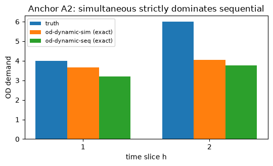
Anchor A2 (“the” anchor): fractional lag, simultaneous strictly dominates
tau = Delta/2 (M0=M1=1/2), H=2 slices, T=3 intervals, truth (4,6),
prior (3,3), V=W=I. The simultaneous solve lets later counts c_2, c_3
REVISE slice 1 through the lag entry; the sequential solve freezes slice 1
from c_1 alone once made. Exact rationals (Cascetta et al.’s own algebra,
recomputed via fractions.Fraction, not quoted from the paper).
m2 = _tensor(0.5, 0.5)
n_intervals2 = 3
truth_a2 = np.array([[4.0], [6.0]])
counts_a2 = predict_interval_counts(m2, truth_a2, n_intervals2)
print(f"predicted interval counts : {counts_a2.reshape(-1)}")
assert np.allclose(counts_a2.reshape(-1), [2.0, 5.0, 3.0])

prior_a2 = np.array([[3.0], [3.0]])
w2, v2 = np.ones((2, 1)), np.ones((3, 1))
sim_a2 = _sim(m2, counts_a2, prior_a2, w2, v2, n_intervals2).reshape(-1)
seq_a2 = _seq(m2, counts_a2, prior_a2, w2, v2, n_intervals2).reshape(-1)

# Exact simultaneous closed form: (I + A'A) d = z + A'c, solved over the rationals.
half = Fraction(1, 2)
a_rows = [[half, Fraction(0)], [half, half], [Fraction(0), half]]
ztc = [Fraction(3), Fraction(3)]
for t in range(3):
    for h in range(2):
        ztc[h] += a_rows[t][h] * Fraction(int(counts_a2[t, 0]))
ata = [[sum(a_rows[t][i] * a_rows[t][j] for t in range(3)) for j in range(2)] for i in range(2)]
hmat = [[ata[i][j] + (1 if i == j else 0) for j in range(2)] for i in range(2)]
det = hmat[0][0] * hmat[1][1] - hmat[0][1] * hmat[1][0]
sim_exact = [
    (hmat[1][1] * ztc[0] - hmat[0][1] * ztc[1]) / det,
    (hmat[0][0] * ztc[1] - hmat[1][0] * ztc[0]) / det,
]
print(f"simultaneous (exact) : {sim_exact}  = {[float(x) for x in sim_exact]}")
assert sim_exact == [Fraction(128, 35), Fraction(142, 35)]
assert np.allclose(sim_a2, [float(x) for x in sim_exact], atol=1e-12)

# Exact sequential: d_1 from c_1 alone (lag 0), then d_2 from c_2 minus frozen d_1 (lag 1).
d1 = (Fraction(3) + half * Fraction(2)) / (1 + half * half)
resid2 = Fraction(5) - half * d1
d2 = (Fraction(3) + half * resid2) / (1 + half * half)
print(f"sequential (exact)   : {[d1, d2]}  = {[float(d1), float(d2)]}")
assert [d1, d2] == [Fraction(16, 5), Fraction(94, 25)]
assert np.allclose(seq_a2, [float(d1), float(d2)], atol=1e-12)

# The headline: simultaneous strictly dominates sequential, componentwise vs truth.
err_sim = np.abs(sim_a2 - truth_a2.reshape(-1))
err_seq = np.abs(seq_a2 - truth_a2.reshape(-1))
print(f"|error| simultaneous : {err_sim}")
print(f"|error| sequential   : {err_seq}")
assert np.all(err_sim < err_seq)
predicted interval counts : [2. 5. 3.]
simultaneous (exact) : [Fraction(128, 35), Fraction(142, 35)]  = [3.657142857142857, 4.057142857142857]
sequential (exact)   : [Fraction(16, 5), Fraction(94, 25)]  = [3.2, 3.76]
|error| simultaneous : [0.34285714 1.94285714]
|error| sequential   : [0.8  2.24]
End to end: two-route, all three T2d units, certified
The public run_dynamic_estimation_experiment API runs prior-profile,
od-dynamic-sim, and od-dynamic-seq on the SAME within-day task and
certifies every checkpoint through DynamicODCertifier: od-dynamic-sim
must strictly beat both od-dynamic-seq and prior-profile on the
descriptive od_rmse — the efficiency ordering Anchor A2 established above,
now confirmed on a real assignment-derived task, not a hand-built tensor.
sc = two_route_scenario(sue_theta=None)
print(f"scenario      : {sc.name}")
print(f"content hash  : {sc.content_hash()[:16]}…")
card = {
    "sensors": {"kind": "explicit", "links": [3]},
    "heldout": {"kind": "explicit", "links": [2]},
    "n_slices": 3, "slice_length": 2.0, "n_days": 12, "noise": "poisson",
    "prior": {"kind": "stale", "cv": 0.3},
}
result = run_dynamic_estimation_experiment(
    sc,
    [DynamicPriorBaseline(), SimultaneousDynamicGLSEstimator(), SequentialDynamicGLSEstimator()],
    Budget(sp_calls=2000), seed=1, macroreps=4, estimation=card,
)
finals = {r["estimator"]: r for r in result.rows if r["macrorep"] == 0}
for name in ("prior-profile", "od-dynamic-sim", "od-dynamic-seq"):
    row = finals[name]
    print(f"{name:16s} od_feasible={row['od_feasible']:.0f}  od_rmse={row['od_rmse']:.4f}  "
          f"heldout_count_rmse={row['heldout_count_rmse']:.4f}")
    assert row["od_feasible"] == 1.0
    assert np.isfinite(float(row["heldout_count_rmse"]))
assert result.manifest["identifiability"]["linear_identifiable"] is True
assert finals["od-dynamic-sim"]["od_rmse"] < finals["od-dynamic-seq"]["od_rmse"]
assert finals["od-dynamic-sim"]["od_rmse"] < finals["prior-profile"]["od_rmse"]
scenario      : tworoute
content hash  : 1ac534dfed2698fb…
prior-profile    od_feasible=1  od_rmse=0.7693  heldout_count_rmse=1.9246
od-dynamic-sim   od_feasible=1  od_rmse=0.2389  heldout_count_rmse=1.7798
od-dynamic-seq   od_feasible=1  od_rmse=0.5522  heldout_count_rmse=1.8667
Visualize
tabench.viz draws a road Network’s per-LINK flows; the od-dynamic
artifact is a per-SLICE demand PROFILE for one OD pair, a different shape
entirely, so this notebook plots the certified per-slice profile directly
(a house profile plot, not tabench.viz) — Anchor A2’s exact simultaneous
and sequential estimates against the truth.
import matplotlib.pyplot as plt

fig, ax = plt.subplots(figsize=(5.5, 3.4))
slices = np.arange(1, 3)
width = 0.25
ax.bar(slices - width, truth_a2.reshape(-1), width, label="truth")
ax.bar(slices, sim_a2, width, label="od-dynamic-sim (exact)")
ax.bar(slices + width, seq_a2, width, label="od-dynamic-seq (exact)")
ax.set_xticks(slices)
ax.set_xlabel("time slice h")
ax.set_ylabel("OD demand")
ax.set_title("Anchor A2: simultaneous strictly dominates sequential")
ax.legend(fontsize=8)
fig.tight_layout()
display(fig)
plt.close(fig)
Takeaways & pointers
Certified, not self-reported. Anchors A1/A2 were recomputed as exact rationals in-cell; the end-to-end two-route run was certified by
DynamicODCertifierinsiderun_dynamic_estimation_experiment, never from a self-report.The efficiency ordering is real, not asymptotic folklore. Anchor A2 proves it exactly on a hand-built tensor; the end-to-end run confirms the SAME ordering (
sim < seq < prior) on a real assignment-derived task.prior-profileis a first-class competitor. It is the baseline both GLS variants must beat (ADR-023covers: [od-dynamic-sim, od-dynamic-seq, prior-profile]).Where next. the static-T2 sibling this reduces to under integer lag
gls(Anchor A1, verified exactly above); the spatial-covariance estimatorod-kalman; the lineage in the model compendium.