`vi-asym` — Asymmetric variational-inequality UE (Dafermos 1980 / Smith 1979)¶

What. When link costs are non-separable and asymmetric — t(v) = t_BPR(v) + C v with C ≠ Cᵀ — no Beckmann potential exists, so the equilibrium is defined only by the variational inequality ⟨t(v*), v − v*⟩ ≥ 0. vi-asym solves it by Dafermos diagonalization (freeze the coupling, solve the separable UE by Frank–Wolfe, repeat) ([dafermos1980traffic], docs/REFERENCES.md).

Why it is in the benchmark. It is the VI branch beyond optimization (ADR-011): the equilibrium is a flow no Beckmann/Frank–Wolfe solver can reach. See the model compendium and docs/ARCHITECTURE.md (P1).

Scope. Runs on the built-in asymmetric two-route anchor (demand 10, c13 = 0.5, c31 = 0.2) and certifies the VI residual.

How this notebook is graded¶

A notebook never claims a number it does not compute in that cell. Every scored quantity below is recomputed live by the P1 Evaluator from the flows the model emitted, in the cell where it is claimed. Model self-reports are shown only as provenance and diffed against the certificate as an honesty check, exactly as the harness treats them (README, Certified, not self-reported).

# Setup. `vi-asym` is a core model: a plain `pip install -e .` suffices — no
# optional extra, so no guard cell. The inline backend is Agg-based (headless CI
# renders into the notebook); NEVER matplotlib.use("Agg") in-kernel — it silently
# suppresses inline figure capture.
%matplotlib inline
import numpy as np

from tabench import (
    AsymmetricVIModel,
    Budget,
    Evaluator,
    RngBundle,
    Trace,
    vi_two_route_scenario,
    viz,
)

The scenario¶

Two disjoint 2-link routes whose congestible legs interact ASYMMETRICALLY (C[1,3] = 0.5 ≠ 0.2 = C[3,1]), so no Beckmann potential exists. The VI equilibrium is f_A* = (1 + (1−c13)·D)/(2 − c13 − c31) = 4.6154, distinct from the plain-UE 5.5. Content-hashed (P2).

scenario = vi_two_route_scenario()
net = scenario.network

print(f"scenario      : {scenario.name}")
print(f"content hash  : {scenario.content_hash()[:16]}…")
print(f"total demand  : {scenario.demand.total}")
print(f"link_interaction set: {scenario.link_interaction is not None}  (asymmetric -> no potential)")

scenario      : vi-tworoute
content hash  : b1c6f69a522efb00…
total demand  : 10.0
link_interaction set: True  (asymmetric -> no potential)

Solve¶

The model contract (CONTRIBUTING.md): a model receives (scenario, budget, rng, trace), records checkpoints, and respects the budget. Budgets are hardware-free (iterations / shortest-path calls; wall-clock is recorded but never the ranking axis, P7). Whatever the model writes into self_report is provenance, not a score.

model = AsymmetricVIModel()
bundle = model.solve(scenario, Budget(iterations=100), RngBundle(0), Trace())

final = bundle.final
print(f"model              : {model.name}")
print(f"emitted flows      : {np.round(final.link_flows, 6)}")
print(f"self-reported resid: {final.self_report['relative_gap']:.3e}  (VI residual, provenance only)")

model              : vi-asym
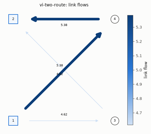
emitted flows      : [4.615385 4.615385 5.384615 5.384615]
self-reported resid: 3.625e-11  (VI residual, provenance only)

Certify (P1)¶

The scored quantity is the VI residual — the normalized relative gap evaluated at the asymmetric cost (a VI gap needs no potential, so the harness reuses the relative-gap machinery with the asymmetric cost map). It is 0 iff v solves the VI. beckmann_objective is NaN (no potential exists). We recompute the closed-form anchor.

evaluator = Evaluator(scenario)
metrics = evaluator.evaluate(final.link_flows)
residual = metrics["relative_gap"]
print(f"certified VI residual : {residual:.3e}")
print(f"feasible              : {metrics['feasible']:.0f}")

assert metrics["feasible"] == 1.0
assert abs(residual) < 1e-8

# Honesty diff (P1).
assert np.isclose(final.self_report["relative_gap"], residual, rtol=1e-6, atol=1e-9)

# Analytic anchor RECOMPUTED: f_A* = (1 + (1-c13) D) / (2 - c13 - c31).
demand = scenario.demand.total
c13, c31 = 0.5, 0.2
f_a = (1.0 + (1.0 - c13) * demand) / (2.0 - c13 - c31)
ref_flows = np.array([f_a, f_a, demand - f_a, demand - f_a])
print(f"VI equilibrium f_A*   : {f_a:.4f}  (recomputed; plain-UE would be {0.5*(demand+1):.1f})")
assert np.allclose(final.link_flows, ref_flows, atol=1e-3)
assert not np.isclose(f_a, 0.5 * (demand + 1.0))  # the asymmetry genuinely shifts it

certified VI residual : 3.625e-11
feasible              : 1
VI equilibrium f_A*   : 4.6154  (recomputed; plain-UE would be 5.5)

Visualize¶

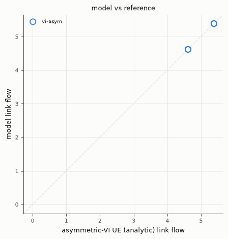
Both figures come from tabench.viz. Left/top: the asymmetric-VI link flows. Right/bottom: the emitted flows against the recomputed VI equilibrium — a flow no Beckmann/Frank–Wolfe solver reaches, because the cost has no potential.

display(viz.plot_network_flows(net, final.link_flows))
display(viz.plot_flow_scatter(("asymmetric-VI UE (analytic)", ref_flows), {"vi-asym": final.link_flows}))

../../_images/bdcde3c34a90363e05fe14935afe9e7eecd72dd6a6371cc5ba161299a7e1a8b1.png

../../_images/f832ebfb4e53009785a9f990e8acc3bd0f5600158ed5fd233d4f8a5b05193128.png

Takeaways & pointers¶

A VI, not an optimization. The residual is a genuine VI gap (no Beckmann potential); the self-report was only diffed against the certificate.
The asymmetry bites. f_A* = 4.6154 ≠ the plain-UE 5.5 — a flow no potential- minimizing solver can reach.
Where next. The separable-cost UE: bfw; the multiclass VI: multiclass; ADR-011 in the model compendium.

vi-asym — Asymmetric variational-inequality UE (Dafermos 1980 / Smith 1979)¶