ctm — Daganzo’s (1994, 1995) Cell Transmission Model

What. ctm is the Godunov cell-transmission scheme for the LWR kinematic-wave model on a triangular fundamental diagram: one link is discretised into n = L / (vf*dt) equal cells at the sanctioned CFL = 1 operating point, so a free-flow vehicle crosses exactly one cell per step and the inter-cell flux is Lebacque’s min(demand, supply). It is a LinkModel on the generic sending/receiving interface (adr-010) — the loader and node models are unchanged, and turning logic is entirely the node models’ job (Daganzo 1995’s network extension).

Why it is in the benchmark. It is the first dynamic-network-loading (DNL) link model — the entry point to the T3 dynamic track, and the workhorse most other DNL/DTA benchmarks compare against. At CFL = 1 the free-flow branch is exact linear advection (zero numerical diffusion); the congested branch resolves a Rankine-Hugoniot backward shock to within one cell. See the model compendium (Daganzo 1994/1995) and the certificate design in docs/design/adr-010-dnl-core.md / adr-015-ctm.md (P1).

Scope. This notebook loads the built-in triangular_bottleneck_dynamic_scenario (a two-link corridor with a capacity bottleneck) through CTMLink and certifies the result. It does not benchmark DNL link models against each other — for that, see the ltm / godunov tutorials.

Canon. [daganzo1994cell], [daganzo1995cell], docs/REFERENCES.md / docs/references.bib.

How this notebook is graded

A notebook never claims a number it does not compute in that cell. Every scored quantity below is recomputed live by the P1 DNLEvaluator from the cumulative link curves the loader emitted, in the cell where it is claimed. Unlike the T1/day-to-day model tutorials, a DNL link model has no self-report to diff against the certificate — NetworkLoader.run() is a deterministic, one-shot forward simulation (no budget, no rng, nothing to converge), so the harness certifies its ONLY output: the emitted cumulative inflow/outflow curves (README, Certified, not self-reported).

# Setup. `ctm` is a core DNL link model: a plain `pip install -e .` suffices —
# no optional extra, so no guard cell. The inline backend is Agg-based (headless
# CI renders into the notebook); NEVER matplotlib.use("Agg") in-kernel — it
# silently suppresses inline figure capture.
%matplotlib inline
import numpy as np

from tabench import (
    CTMLink,
    DNLEvaluator,
    NetworkLoader,
    triangular_bottleneck_dynamic_scenario,
    viz,
)

The scenario

The built-in triangular_bottleneck_dynamic_scenario: a two-link corridor (origin zone 1 → interior node 3 → destination zone 2), symmetric triangular FD vf = w = 1, finite jam density kappa = 4 (so capacity = vf*w*kappa/(vf+w) = 2), feeding a 0.5-capacity sink link. Arrivals start at rate 1.5 — above the sink’s capacity, so a queue backs up the upstream link. Scenarios are frozen and content-hashed (P2) — the hash below is the instance’s identity. (The two kappa = inf point-queue anchors single_link_dynamic_scenario / bottleneck_dynamic_scenario are rejected by CTMLink — a finite jam density is required to model bounded storage / spillback.)

scenario = triangular_bottleneck_dynamic_scenario()
net = scenario.network
dyn = scenario.dynamics
print(f"scenario      : {scenario.name}")
print(f"content hash  : {scenario.content_hash()[:16]}…")
print(f"links         : {net.n_links}  (tail→head: "
      + ", ".join(f"{i}->{j}" for i, j in zip(net.init_node, net.term_node)) + ")")
print(f"link 0 (up)   : vf={dyn.free_speed[0]}, w={dyn.wave_speed[0]}, "
      f"kappa={dyn.jam_density[0]}, capacity={dyn.capacity[0]}, L={dyn.length[0]}")
print(f"link 1 (sink) : vf={dyn.free_speed[1]}, w={dyn.wave_speed[1]}, "
      f"kappa={dyn.jam_density[1]}, capacity={dyn.capacity[1]}, L={dyn.length[1]}")
print(f"grid          : dt={scenario.grid.dt}, n_steps={scenario.grid.n_steps}")
print("task          : deterministic DNL loading (feasibility + conservation + shock)")

scenario      : dnl-triangular-bottleneck
content hash  : d4148843c3292e42…
links         : 2  (tail→head: 1->3, 3->2)
link 0 (up)   : vf=1.0, w=1.0, kappa=4.0, capacity=2.0, L=4.0
link 1 (sink) : vf=1.0, w=1.0, kappa=4.0, capacity=0.5, L=1.0
grid          : dt=1.0, n_steps=12
task          : deterministic DNL loading (feasibility + conservation + shock)

Load the network

The DNL model contract (adr-010): a LinkModel factory + a DynamicScenario go into NetworkLoader, which runs a deterministic sending/receiving time loop and emits cumulative inflow/outflow curves per link — no Budget/RngBundle/Trace, because there is nothing to converge or seed: one forward pass over the grid is the entire computation.

loader = NetworkLoader(scenario, CTMLink)
out = loader.run()
edges = scenario.grid.edges
print(f"link model       : {CTMLink.__name__}")
print(f"cells (link 0)    : {loader.links[0].n_cells}  (L / (vf*dt) = "
      f"{dyn.length[0] / (dyn.free_speed[0] * scenario.grid.dt):.0f})")
print(f"emitted n_in[0]   : {np.round(out.n_in[0, ::4], 3)}  (every 4th edge)")
print(f"emitted n_out[0]  : {np.round(out.n_out[0, ::4], 3)}  (every 4th edge)")
print(f"vehicles in link 0 storage at t={edges[-1]:.0f}: "
      f"{out.n_in[0, -1] - out.n_out[0, -1]:.3f}")

link model       : CTMLink
cells (link 0)    : 4  (L / (vf*dt) = 4)
emitted n_in[0]   : [ 0.  6. 12. 18.]  (every 4th edge)
emitted n_out[0]  : [0. 0. 2. 4.]  (every 4th edge)
vehicles in link 0 storage at t=12: 14.000

Certify (P1) — feasibility, conservation, and the RH-shock anchor

The harness recomputes every certificate from (scenario, out) alone: C0 shape/validity, C1 conservation, C2 capacity respect, C3 storage bounds, C4/C6 free-flow causality, and (Tier-B) C5 the backward-wave envelope. Beyond that structural gate, the arrival rate (1.5) exceeds the sink capacity (0.5), so a Rankine-Hugoniot shock forms at the link-1 boundary once the free-flow front arrives (t = L/vf = 4) and propagates upstream — recomputed here from the two FD branches, not quoted.

metrics = DNLEvaluator(scenario).evaluate(out)
print(f"dnl_feasible            : {metrics['dnl_feasible']:.0f}")
print(f"conservation_residual   : {metrics['conservation_residual']:.3e}")
print(f"storage_residual        : {metrics['storage_residual']:.3e}")
print(f"causality_residual      : {metrics['causality_residual']:.3e}")
print(f"tstt                    : {metrics['tstt']:.3f}")
print(f"total_delay             : {metrics['total_delay']:.3f}")
assert metrics["dnl_feasible"] == 1.0
assert metrics["conservation_residual"] <= 1e-9
assert metrics["storage_residual"] <= 1e-9
assert metrics["causality_residual"] <= 1e-9

# Boundary curves, recomputed from the physical parameters (arrival rate 1.5,
# bottleneck rate 0.5, free-flow front at t = L/vf = 4) — not the point-queue
# formula, the exact CTM boundary curve for a triangular FD at CFL = 1.
expected_n_in = 1.5 * edges                       # uncongested arrival never throttled
expected_n_out = np.maximum(0.0, 0.5 * (edges - 4.0))  # bottleneck-capped exit from t=4
np.testing.assert_allclose(out.n_in[0], expected_n_in, atol=1e-9)
np.testing.assert_allclose(out.n_out[0], expected_n_out, atol=1e-9)
print("boundary curves match the recomputed RH-shock anchor exactly (atol=1e-9)")

# The distinctive CTM result: every congested cell settles at the SUPPLY-side
# root of the FD (k = kappa - q_B/w), recomputed from the FD directly, not
# hand-quoted.
fd0 = scenario.dynamics.fd(0)
k_b = fd0.jam_density - 0.5 / fd0.wave_speed
dx = fd0.free_speed * scenario.grid.dt
density = loader.links[0].occupancy / dx
print(f"congested cells density : {np.round(density, 4)}  (supply-root k_B = {k_b:.4f})")
assert abs(float(fd0.supply_at(np.array([k_b]))[0]) - 0.5) < 1e-9
# Full spillback by t=12: every cell is engulfed by the queue, all at k_B.
np.testing.assert_allclose(density, k_b, atol=1e-9)

dnl_feasible            : 1
conservation_residual   : 0.000e+00
storage_residual        : 0.000e+00
causality_residual      : 0.000e+00
tstt                    : 95.750
total_delay             : 19.750
boundary curves match the recomputed RH-shock anchor exactly (atol=1e-9)
congested cells density : [3.5 3.5 3.5 3.5]  (supply-root k_B = 3.5000)

Visualize

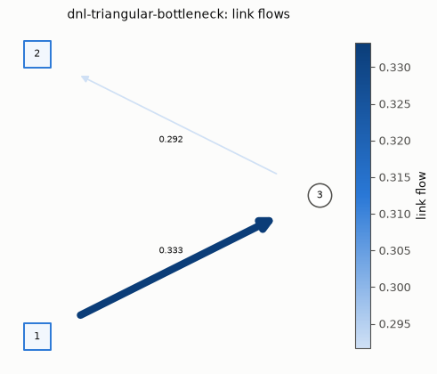
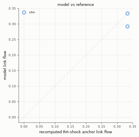
Both figures come from tabench.viz, the house visualizer. Left/top: the certified network with each link coloured/sized by its TIME-AVERAGED flow (n_out(T) / T, the DNL analogue of a static link flow). Right/bottom: the loaded average flow against the recomputed boundary-curve anchor above — the sink link visibly sits at its throttled capacity (0.5), not the uncongested arrival rate.

T = float(edges[-1])
avg_flow = out.n_out[:, -1] / T
ref_avg_flow = np.array([expected_n_out[-1] / T, expected_n_out[-1] / T])

display(viz.plot_network_flows(net, avg_flow))
display(viz.plot_flow_scatter(("recomputed RH-shock anchor", ref_avg_flow), {"ctm": avg_flow}))

Takeaways & pointers

• Certified, not self-reported. DNL link models have nothing to self-report — the boundary curves above ARE the emitted output, and DNLEvaluator recomputes every certificate from them alone.

• CFL = 1 is exact. The free-flow branch is bit-exact linear advection; the congested branch resolves the RH shock to machine precision on this symmetric FD (an asymmetric w < vf FD spreads the shock by O(one cell) — expected scheme physics, why C5 is a non-gating Tier-B residual for CTM).

• Where next. the exact cumulative-curve alternative ltm (no cell alignment required); the smooth non-triangular FD godunov; merges/diverges node-model; the lineage in the model compendium.