vzw-entropy — Van Zuylen & Willumsen’s (1980) entropy-balancing OD estimation

What. vzw-entropy (T2, ADR-002) is the information-minimizing sibling of gls: instead of a quadratic prior/count trade-off, it multiplicatively balances each OD cell in log-space against every sensor’s count via a damped fixed-point iteration — an EXPONENT form, g <- (c/p)^p per sensor, not a linear blend. It is the classical maximum-entropy / minimum-information estimator (biproportional fitting lineage), a genuinely different mathematical family from gls’s quadratic program.

Why it is in the benchmark. Entropy balancing predates gls in the OD estimation literature and is still the default in several commercial packages; its damped multiplicative update converges geometrically to a DIFFERENT fixed point than a linear GLS blend whenever sensors disagree, which this notebook makes an executable, hand-verified fact. See the model compendium (Van Zuylen & Willumsen 1980) and docs/design/adr-002-t2-estimation-certificate.md (P1).

Scope. The exact single-sensor exponent fixed point (one pass vs converged), the damped multi-sensor compromise under mutually inconsistent counts, and the Braess global-basin D=6 recovery.

Canon. [vanzuylen1980most], docs/REFERENCES.md / docs/references.bib.

How this notebook is graded

A notebook never claims a number it does not compute in that cell. Every scored quantity below is recomputed live — the closed-form fixed points are recomputed algebraically in-cell (no trusted digits), and the Braess recovery is recomputed by the P1 ODCertifier from the emitted OD matrix against the harness’s own pinned BFW assignment, never from vzw-entropy’s self-report (README, Certified, not self-reported).

# Setup. `vzw-entropy` is a core estimator: a plain `pip install -e .`
# suffices — no optional extra, so no guard cell. The inline backend is
# Agg-based (headless CI renders into the notebook); NEVER
# matplotlib.use("Agg") in-kernel — it silently suppresses inline capture.
%matplotlib inline
import numpy as np

from tabench import (
    Budget,
    Demand,
    ODCertifier,
    RngBundle,
    Trace,
    VZWEntropyEstimator,
    braess_scenario,
    two_route_scenario,
    viz,
)
from tabench.core.rng import SOURCE_OBSERVATION
from tabench.estimation import ODTrace, vzw_balance
from tabench.estimation.base import EstimationTask
from tabench.models.frank_wolfe import BiconjugateFrankWolfeModel
from tabench.observe.levels import LinkCounts

BRAESS_TRUTH = np.array([4.0, 2.0, 2.0, 2.0, 4.0])  # UE(D=6), recomputed below
TWOROUTE_TRUTH = np.array([2.5, 2.5, 1.5, 1.5])  # UE(D=4), recomputed below

# Analytic anchors recomputed, never quoted: pin both by an independent
# high-precision BFW solve before EITHER constant is used as a data-generating
# truth anywhere below.
def _pinned_ue(scenario):
    trace = Trace()
    BiconjugateFrankWolfeModel().solve(
        scenario, Budget(iterations=5000, target_relative_gap=1e-10), RngBundle(0), trace
    )
    return trace.final.link_flows

np.testing.assert_allclose(_pinned_ue(braess_scenario(6.0)), BRAESS_TRUTH, atol=1e-6)
np.testing.assert_allclose(_pinned_ue(two_route_scenario(sue_theta=None)), TWOROUTE_TRUTH, atol=1e-6)

The exponent fixed point: one pass vs geometric convergence

Single pair, single sensor on route A (p_a = 2.5/4 = 0.625, count c=2.5). One damped pass gives T = (c/p)^p, NOT the linear-blend result c/p a gls-style update would give in one step; the geometric limit over many passes IS the exact fixed point c/p = 4.0.

p_a = TWOROUTE_TRUTH[0] / 4.0  # route-A proportion, recomputed
count = TWOROUTE_TRUTH[0]

best_g1, traj1, consistent1 = vzw_balance(
    np.array([1.0]), np.array([[p_a]]), np.array([count]), n_passes=1
)
print(f"one-pass estimate : {best_g1[0]:.6f}  (c/p)^p = {(count / p_a) ** p_a:.6f}")
assert np.isclose(best_g1[0], (count / p_a) ** p_a, atol=1e-12)
assert consistent1 is False  # one pass has not yet reached the fixed point
assert len(traj1) == 2  # prior + one update

best_g60, _, consistent60 = vzw_balance(
    np.array([1.0]), np.array([[p_a]]), np.array([count]), n_passes=60
)
print(f"60-pass estimate   : {best_g60[0]:.6f}  (fixed point c/p = {count / p_a:.6f})")
assert np.isclose(best_g60[0], count / p_a, atol=1e-9)
assert np.isclose(best_g60[0], 4.0, atol=1e-9)
assert consistent60 is True

one-pass estimate : 2.378414  (c/p)^p = 2.378414
60-pass estimate   : 4.000000  (fixed point c/p = 4.000000)

Mutually inconsistent sensors: a damped compromise, not oscillation

Two sensors on the SAME pair, at odds (c_a=3.0 on route A’s proportion, c_b=1.0 on route B’s) — no single demand satisfies both exactly. The damped log-space update converges to a compromise fixed point, recomputed here exactly via the sequential single-link recursion.

p_b = TWOROUTE_TRUTH[2] / 4.0  # route-B proportion, recomputed
c_a, c_b = 3.0, 1.0
best_g, _, consistent = vzw_balance(
    np.array([1.0]), np.array([[p_a], [p_b]]), np.array([c_a, c_b]), n_passes=400
)
# Sequential log-space fixed point of the two damped single-link updates
# x <- (1-p)*x + p*log(c/p), applied for sensor a then b:
t_a, t_b = np.log(c_a / p_a), np.log(c_b / p_b)
x_star = ((1 - p_b) * p_a * t_a + p_b * t_b) / (1 - (1 - p_a) * (1 - p_b))
print(f"compromise estimate : {best_g[0]:.6f}")
print(f"closed-form exp(x*) : {np.exp(x_star):.6f}")
assert np.isclose(best_g[0], np.exp(x_star), atol=1e-6)
assert consistent is False  # mutually inconsistent -> residual above tolerance

compromise estimate : 3.599232
closed-form exp(x*) : 3.599232

Braess: global-basin recovery from D=5.5

braess_scenario(6.0) is the D=6 Braess network, frozen and content-hashed (P2). From a prior D=5.5 — inside the global basin (see spiess for the D=4 SPURIOUS-basin caveat this network also has) — full noiseless sensors let vzw-entropy recover the true D=6.

sc = braess_scenario(6.0)
print(f"scenario      : {sc.name}")
print(f"content hash  : {sc.content_hash()[:16]}…")

prior_matrix = np.zeros((2, 2))
prior_matrix[0, 1] = 5.5
ds = LinkCounts(np.arange(5), 1, "none").observe(
    sc, BRAESS_TRUTH, RngBundle(0).generator(SOURCE_OBSERVATION)
)
task = EstimationTask(
    name="t", network=sc.network, prior=Demand(prior_matrix), dataset=ds,
    identifiability={}, scenario_hash=sc.content_hash(), seed=0,
)
trace = ODTrace()
VZWEntropyEstimator(k_inner=120, outer_iters=80).estimate(
    task, Budget(sp_calls=10**9, iterations=200), RngBundle(0), trace
)
recovered = trace.final.od_matrix[0, 1]
print(f"recovered D : {recovered:.4f}  (truth: 6.0, off prior: 5.5)")
assert abs(recovered - 6.0) < 1e-3

certifier = ODCertifier(
    sc, np.arange(5), np.array([], dtype=np.int64),
    BRAESS_TRUTH[None, :], BRAESS_TRUTH[[]][None, :], BRAESS_TRUTH,
    {"linear_identifiable": True},
)
metrics = certifier.certify(trace.final.od_matrix)
print(f"certified od_rmse : {metrics['od_rmse']:.4e}")
assert metrics["od_feasible"] == 1.0
assert metrics["od_rmse"] < 1e-3

scenario      : braess
content hash  : cf00f411cdccec88…
recovered D : 6.0000  (truth: 6.0, off prior: 5.5)
certified od_rmse : 0.0000e+00

Visualize

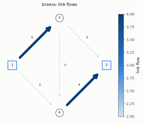
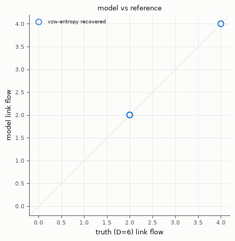
tabench.viz draws the road Network’s link flows for the recovered Braess demand against the truth (the same certified OD matrix from the cell above, re-assigned).

recovered_matrix = trace.final.od_matrix
from tabench import Scenario
recovered_trace = Trace()
BiconjugateFrankWolfeModel().solve(
    Scenario("recovered", sc.network, Demand(recovered_matrix), family=sc.family),
    Budget(iterations=5000, target_relative_gap=1e-10), RngBundle(0), recovered_trace,
)
display(viz.plot_network_flows(sc.network, BRAESS_TRUTH))
display(viz.plot_flow_scatter(
    ("truth (D=6)", BRAESS_TRUTH),
    {"vzw-entropy recovered": recovered_trace.final.link_flows},
))

Takeaways & pointers

• Certified, not self-reported. The Braess od_rmse above came from ODCertifier’s own re-assignment of the emitted OD matrix, never from vzw-entropy’s internal proportions.

• The exponent form is distinctive. One damped pass gives (c/p)^p, not a linear gls-style blend — verified exactly above, not asserted.

• Where next. the quadratic-tradeoff sibling on the SAME network gls; the count-only end of the spectrum spiess; the lineage in the model compendium.