dtd-stochastic — Cascetta’s (1989) stochastic-process day-to-day model

What. The benchmark’s first genuinely stochastic day-to-day model: each day a finite population of travellers samples routes multinomially from the Dial logit fractions at the perceived costs, and memory smooths toward the realized experienced costs. The daily flows never converge; the emitted flow is the burnt-in time average.

Why it is in the benchmark. It witnesses honestly that the stationary MEAN is only approximately SUE at finite population: the certified residual floors at O(bias + SE) (tolerances 0.05, not 1e-5), the daily flows keep an O(1/√N) deviation (Davis & Nihan 1993), and the time average converges by the ergodic theorem. See the model compendium and the certificate design in docs/ARCHITECTURE.md (P1).

Scope. Runs the process on a built-in scenario and certifies the result; it does not benchmark day-to-day models against each other. Reference: Cascetta, E. (1989), Transportation Research Part B 23(1).

Canon. [cascetta1989stochastic], docs/REFERENCES.md / docs/references.bib.

How this notebook is graded

A notebook never claims a number it does not compute in that cell. Every scored quantity below is recomputed live by the P1 Evaluator from the flows the model emitted, in the cell where it is claimed. Model self-reports (the per-day gap/residual, the Lyapunov value) are shown only as provenance and diffed against the certificate, exactly as the harness treats them (README, Certified, not self-reported).

# Setup. `dtd-stochastic` is a core day-to-day model: a plain `pip install -e .` suffices —
# no optional extra, so no guard cell. The inline backend is Agg-based (headless CI
# renders into the notebook); NEVER matplotlib.use("Agg") in-kernel — it silently
# suppresses inline figure capture.
%matplotlib inline
import numpy as np

from tabench import (
    Budget,
    CascettaStochasticProcessModel,
    Evaluator,
    RngBundle,
    Trace,
    two_route_scenario,
    viz,
)

The scenario

The built-in two-route logit-SUE anchor (demand 4, dispersion θ=0.5): route A cost 2+f_A, route B cost 1.5+2 f_B. Its rest point is the binary-logit stochastic user equilibrium, recomputed analytically in the certify cell — NOT the deterministic Wardrop UE.

scenario = two_route_scenario()
net = scenario.network
print(f"scenario      : {scenario.name}")
print(f"content hash  : {scenario.content_hash()[:16]}…")
print(f"links         : {net.n_links}  (tail→head: "
      + ", ".join(f"{i}->{j}" for i, j in zip(net.init_node, net.term_node)) + ")")
print(f"total demand  : {scenario.demand.total}")
print("task          : logit SUE, θ=0.5")

scenario      : tworoute
content hash  : 9b98e58b339b702f…
links         : 4  (tail→head: 1->3, 3->2, 1->4, 4->2)
total demand  : 4.0
task          : logit SUE, θ=0.5

Run the adjustment process

The model contract (CONTRIBUTING.md): a model receives (scenario, budget, rng, trace) and records one checkpoint per day — here a budget iteration is a day. Everything the model writes into self_report (the per-day gap/residual, the Lyapunov value) is provenance, not a score.

bundle_trace = Trace()
model = CascettaStochasticProcessModel(
    smoothing_weight=0.3, population_scale=25.0, burn_in_days=500
)
model.solve(scenario, Budget(iterations=3000), RngBundle(0), bundle_trace)
final = bundle_trace.final
print(f"model            : {model.name}")
print(f"days simulated   : {final.coords.iterations}  "
      f"({final.coords.sp_calls} shortest-path calls)")
print(f"emitted flows    : {np.round(final.link_flows, 6)}")
print(f"self-reported residual: {final.self_report['sue_fixed_point_residual']:.3e}  (provenance only)")

model            : dtd-stochastic
days simulated   : 3000  (6000 shortest-path calls)
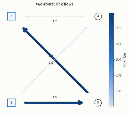
emitted flows    : [2.296176 2.296176 1.703824 1.703824]
self-reported residual: 7.201e-03  (provenance only)

Certify (P1) — a stationary distribution, honestly

The harness recomputes the Dial-STOCH residual of the burnt-in time average. Because the population is finite, the residual floors at O(bias + SE) — the tolerances are 0.05, not machine ε, and the notebook certifies exactly that honest floor plus the persistent daily variability that makes equilibrium a distribution, not a fixed point.

from scipy.optimize import brentq
evaluator = Evaluator(scenario)
metrics = evaluator.evaluate(final.link_flows)
residual = metrics["sue_fixed_point_residual"]
print(f"certified SUE residual : {residual:.3e}  (floors at O(bias+SE), not machine ε)")
print(f"feasible               : {metrics['feasible']:.0f}")
assert metrics["feasible"] == 1.0
assert residual < 0.05  # finite-population floor — NOT solver precision
assert metrics["relative_gap"] > 0.01

# The burnt-in TIME AVERAGE lands within 0.05 of the analytic logit SUE (θ=0.5).
def _resid(f_a):
    c_a, c_b = 2.0 + f_a, 1.5 + 2.0 * (4.0 - f_a)
    return f_a - 4.0 / (1.0 + np.exp(0.5 * (c_a - c_b)))
f_a = brentq(_resid, 0.0, 4.0, xtol=1e-12)
ref_flows = np.array([f_a, f_a, 4.0 - f_a, 4.0 - f_a])
assert np.allclose(final.link_flows, ref_flows, atol=0.05)

# DISTINCTIVE: equilibrium is a STATIONARY DISTRIBUTION, not a fixed point. The daily
# flows keep an O(1/√N) deviation from the mean even while the time-average residual is
# small; the deviation shrinks as the population grows (Davis & Nihan 1993).
dev_tail = [s.self_report["daily_flow_deviation"] for s in list(bundle_trace)[-100:]]
print(f"tail daily deviation   : {np.mean(dev_tail):.3f}  (persists at finite N)")
assert np.mean(dev_tail) > 0.05
print(f"stationary window_days : {final.self_report['window_days']:.0f}  (days backing the average)")
assert final.self_report["window_days"] == 2500.0
# Honesty (P1): the self-reported residual equals the harness certificate.
assert np.isclose(
    final.self_report["sue_fixed_point_residual"], residual, rtol=1e-9, atol=1e-12
)

certified SUE residual : 7.201e-03  (floors at O(bias+SE), not machine ε)
feasible               : 1
tail daily deviation   : 0.182  (persists at finite N)
stationary window_days : 2500  (days backing the average)

Visualize

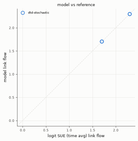
Both figures come from tabench.viz, the house visualizer — every plotted number is one certified above. Left/top: the certified terminal link flows on the network. Right/bottom: the emitted flows against the fixed point recomputed in the certify cell — points on the y = x guide mean the day-to-day process settled on it link-for-link.

# Certified terminal flows on the network (house style via tabench.viz).
display(viz.plot_network_flows(net, final.link_flows))

# Emitted flows vs the logit SUE (time avg) recomputed above (off-diagonal == not settled).
display(viz.plot_flow_scatter(("logit SUE (time avg)", ref_flows), {"dtd-stochastic": final.link_flows}))

Takeaways & pointers

• Certified, not self-reported. The residual and the anchor came from Evaluator at the loose finite-population tolerance; the self-report matched the certificate, so the O(bias+SE) floor is honestly scored, never a false accept.

• The day-to-day signature is the point. A UE/SUE solver gives you the fixed point; a day-to-day model gives you the adjustment path to it.

• Where next. the deterministic-in-the-mean limit dtd-horowitz; the unifying framework dtd-unifying; the lineage in the model compendium.