bfw — Bi-conjugate Frank–Wolfe on the Braess network

What. bfw is Mitradjieva & Lindberg’s (2013) bi-conjugate Frank–Wolfe solver for the deterministic user-equilibrium (UE) traffic assignment problem ([mitradjieva2013stiff] in the verified canon, docs/REFERENCES.md / docs/references.bib). Plain Frank–Wolfe zig-zags in its tail because one scalar step is shared by all OD pairs; BFW replaces the raw all-or-nothing search point with a convex combination of the AON point and the previous two search points, chosen conjugate with respect to the diagonal Beckmann Hessian — killing the tail while keeping link-only O(m) storage (no path or bush enumeration).

Why it is in the benchmark. It is the workhorse of the convergence race (link-based → conjugate → path/bush-based) and the repo’s default high-precision UE reference; see its entry in the model compendium and the certificate design in docs/ARCHITECTURE.md (P1).

Scope. This notebook runs bfw on the built-in Braess scenario (5 links, one OD pair, no download) and certifies the result. It does not benchmark solver families against each other — for that, see the fw / cfw / tapas tutorials and demos/demo_quickstart.py.

How this notebook is graded

A notebook never claims a number it does not compute in that cell. Every scored quantity below — the certified relative gap, feasibility, the analytic anchor check — is recomputed live by the P1 evaluator from the flows the model emitted, in the cell where it is claimed. Model self-reports are shown only as provenance and diffed against the certificate as an honesty check, exactly as the harness treats them (README, Certified, not self-reported).

# Setup. `bfw` is a core model: a plain `pip install -e .` suffices — no optional
# extra, so no guard cell. (Notebooks for torch/sumo/dtalite models carry a guard
# cell here that raises politely when the extra is missing.)
#
# The inline backend is Agg-based: figures render headlessly into the notebook, so
# CI can execute tutorials without a display. NEVER matplotlib.use("Agg") in-kernel
# — it silently suppresses inline figure capture.
%matplotlib inline
import numpy as np

from tabench import (
    BiconjugateFrankWolfeModel,
    Budget,
    Evaluator,
    RngBundle,
    Trace,
    braess_scenario,
    viz,
)

The scenario

The built-in Braess network: 4 nodes, 5 links, a single OD pair (1 → 2) with demand 6. Scenarios are frozen and content-hashed (P2) — the hash printed below is the identity of the benchmark instance, so a silently edited network cannot masquerade as it.

scenario = braess_scenario()
net = scenario.network

print(f"scenario      : {scenario.name}")
print(f"content hash  : {scenario.content_hash()[:16]}…")
print(f"links         : {net.n_links}  (tail→head: "
      + ", ".join(f"{i}->{j}" for i, j in zip(net.init_node, net.term_node)) + ")")
print(f"total demand  : {scenario.demand.total}")

scenario      : braess
content hash  : cf00f411cdccec88…
links         : 5  (tail→head: 1->3, 1->4, 3->4, 3->2, 4->2)
total demand  : 6.0

Solve

The model contract (CONTRIBUTING.md): a model receives (scenario, budget, rng, trace), records checkpoints, and respects the budget. Budgets are hardware-free (iterations / shortest-path calls; wall-clock is recorded but never the ranking axis, P7). Whatever the model writes into self_report is provenance, not a score.

model = BiconjugateFrankWolfeModel()
bundle = model.solve(scenario, Budget(iterations=50), RngBundle(0), Trace())

final = bundle.final
print(f"model            : {model.name}")
print(f"budget spent     : {final.coords.iterations} iterations, "
      f"{final.coords.sp_calls} shortest-path calls")
print(f"checkpoints      : {len(bundle.trace.checkpoints)}")
print(f"emitted flows    : {np.round(final.link_flows, 6)}")
print(f"self-reported gap: {final.self_report['relative_gap']:.3e}  (provenance only)")

model            : bfw
budget spent     : 3 iterations, 4 shortest-path calls
checkpoints      : 3
emitted flows    : [4. 2. 2. 2. 4.]
self-reported gap: -2.060e-16  (provenance only)

Certify (P1)

The harness, never the model, computes every scored metric: the relative gap is a property of (link_flows, scenario), recomputed here by the same Evaluator that scores every model in the benchmark — a 1975 Frank–Wolfe and a 2025 GNN share this certificate. We also recompute the analytic Braess anchor in this cell rather than quoting it: at UE the flows are (4, 2, 2, 2, 4) and every used route costs 92 (pinned in tests/test_braess.py and docs/VALIDATION.md).

evaluator = Evaluator(scenario)
metrics = evaluator.evaluate(final.link_flows)

certified_gap = metrics["relative_gap"]
print(f"certified relative gap : {certified_gap:.3e}")
print(f"feasible               : {metrics['feasible']:.0f}")
print(f"Beckmann objective     : {metrics['beckmann_objective']:.6f}")

# Equilibrium reached at solver precision, and the demand audit passed.
assert metrics["feasible"] == 1.0
assert abs(certified_gap) < 1e-10

# Honesty diff (P1): the white box's self-report must match the certificate.
assert np.isclose(final.self_report["relative_gap"], certified_gap, rtol=1e-9, atol=1e-12)

# Analytic anchor, recomputed in-cell: flows (4,2,2,2,4); at UE every used route
# costs 92, so TSTT / demand equals the route time.
ref_flows = np.array([4.0, 2.0, 2.0, 2.0, 4.0])
assert evaluator.evaluate(ref_flows)["relative_gap"] < 1e-6
assert np.allclose(final.link_flows, ref_flows, atol=1e-4)
route_time = metrics["tstt"] / scenario.demand.total
print(f"route time (TSTT/D)    : {route_time:.6f}  (analytic UE: 92)")
assert np.isclose(route_time, 92.0, atol=1e-4)

# Certify EVERY checkpoint the same way — this trace feeds the visual below, so the
# plotted flows are certificate data, not self-reports.
trace_iters = [c.coords.iterations for c in bundle.trace.checkpoints]
trace_gaps = [evaluator.evaluate(c.link_flows)["relative_gap"] for c in bundle.trace.checkpoints]
for it, gap in zip(trace_iters, trace_gaps):
    print(f"  iteration {it}: certified gap {gap:.3e}")

certified relative gap : -2.060e-16
feasible               : 1
Beckmann objective     : 386.000008
route time (TSTT/D)    : 92.000000  (analytic UE: 92)
  iteration 1: certified gap 1.912e-01
  iteration 2: certified gap 2.125e-01
  iteration 3: certified gap -2.060e-16

Visualize

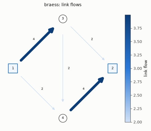
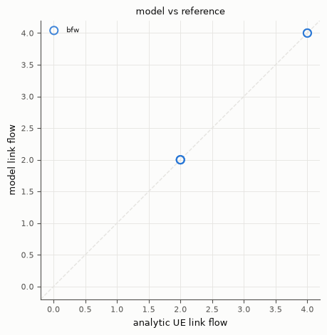
Both figures come from tabench.viz, the house visualizer — one visual style across every tutorial, and every plotted number is a quantity certified above. Left/top: the certified equilibrium link flows on the Braess diamond (link width and colour encode flow; the 3→4 bypass carries the paradox). Right/bottom: the emitted bfw flows against the analytic UE recomputed in the previous cell — every point sits on the y = x guide, so the solver reproduced the certified equilibrium link-for-link.

# tabench.viz returns library-style Figures (not pyplot-registered); display each inline.
# Certified equilibrium flows on the network (house style via tabench.viz).
display(viz.plot_network_flows(net, final.link_flows))

# Emitted flows vs the analytic UE anchor recomputed above: on-diagonal == reproduced.
display(viz.plot_flow_scatter(("analytic UE", ref_flows), {"bfw": final.link_flows}))

Takeaways & pointers

• Certified, not self-reported. The gap above came from Evaluator, recomputed from the emitted flows in this notebook — the self-report was only diffed against it.

• BFW earns its place: it reaches machine-precision UE on Braess in the handful of iterations printed above; on Winnipeg it heads the solver ladder (see the README table — run it, don’t quote it).

• Where next.

  • The tail it fixes: fw · the one-conjugate variant: cfw · the simple baseline: msa.

  • Lineage and “what it does differently”: the Mitradjieva & Lindberg (2013) entry in the model compendium.

  • Oracle validation (best-known flows, cross-solver agreement): docs/VALIDATION.md.

  • The full matrix: tabench run --scenario siouxfalls --models fw,cfw,bfw or run_experiment(...) as in demos/demo_quickstart.py.