vickrey — Vickrey’s (1969) single-bottleneck departure-time equilibrium

What. vickrey is the analytical departure-TIME equilibrium at a single deterministic-queue (point-queue) bottleneck: commuters choose WHEN to depart, trading queueing delay against early/late schedule-delay penalties around a preferred arrival time t*. Its closed form is a Wardrop-style equal-cost condition on the time axis instead of the route axis — the entry point of the benchmark’s analytical dynamic-UE (DUE) track.

Why it is in the benchmark. It is the first model to make departure time itself an equilibrium choice variable, and proves the pure-queueing user equilibrium wastes exactly a factor of two versus the system optimum (Price of Anarchy = 2) — a closed-form, machine-checkable result. See the model compendium (Vickrey 1969) (P1).

Scope. This notebook runs the closed-form UE and SO schedules on the built-in worked instance and certifies both. It does not benchmark departure- time solvers against each other — this track ships only the closed form.

Canon. [vickrey1969congestion], docs/REFERENCES.md / docs/references.bib.

How this notebook is graded

A notebook never claims a number it does not compute in that cell. Every scored quantity below is recomputed live by the P1 BottleneckEvaluator from the emitted cumulative departure curve R(t) alone — the deterministic point queue, each used departure time’s generalized cost, and the equilibrium gap are all reconstructed from R(t), never taken from the solver’s own r_early/t1/C* provenance (README, Certified, not self-reported).

# Setup. `vickrey` is a core model: a plain `pip install -e .` suffices — no
# optional extra, so no guard cell. The inline backend is Agg-based (headless
# CI renders into the notebook); NEVER matplotlib.use("Agg") in-kernel — it
# silently suppresses inline figure capture.
%matplotlib inline
import numpy as np

from tabench import (
    BottleneckEvaluator,
    so_closed_form,
    ue_closed_form,
    vickrey_worked_scenario,
)

The scenario

The built-in worked instance: N=6000 travelers, bottleneck capacity s=3000/h, schedule-delay slopes alpha=1, beta=0.5, gamma=2, preferred arrival t*=9. BottleneckScenario is frozen and content-hashed (P2).

scenario = vickrey_worked_scenario()
print(f"scenario      : {scenario.name}")
print(f"content hash  : {scenario.content_hash()[:16]}…")
print(f"N={scenario.n_travelers}, s={scenario.capacity}, alpha={scenario.alpha}, "
      f"beta={scenario.beta}, gamma={scenario.gamma}, t*={scenario.t_star}")
print(f"equilibrium cost C* (property) : {scenario.equilibrium_cost}")
print("task          : departure-time user equilibrium vs system optimum")

scenario      : vickrey-worked
content hash  : a4ef2d96f75397f1…
N=6000.0, s=3000.0, alpha=1.0, beta=0.5, gamma=2.0, t*=9.0
equilibrium cost C* (property) : 0.8
task          : departure-time user equilibrium vs system optimum

Solve

No Budget/RngBundle/Trace — the closed forms are pure functions of the scenario, each emitting a BottleneckSchedule (a cumulative departure curve R(t) on a time grid, the P1-certifiable artifact).

ue = ue_closed_form(scenario)
so = so_closed_form(scenario)
print(f"UE provenance : {ue.provenance}")
print(f"SO provenance : {so.provenance}")

UE provenance : {'r_early': 6000.0, 'r_late': 1000.0, 't1': 7.4, 't2': 9.4, 't_n': 8.2, 'equilibrium_cost': 0.8}
SO provenance : {'rate': 3000.0, 't1': 7.4, 't2': 9.4, 'queue': 0.0}

Certify (P1) — the equal-cost condition, honestly

The harness reconstructs the deterministic point queue from R(t) alone, recomputes each used departure time’s generalized cost by inverting BOTH the arrival and served curves (per-traveler, not per-grid-step — a start-of-step sample would let a burst dump falsely certify), and scores equilibrium_gap = (max cost - min cost) / C*: zero iff every used departure time is equally costly (a true UE), positive otherwise.

evaluator = BottleneckEvaluator(scenario)
m_ue = evaluator.certify(ue)
m_so = evaluator.certify(so)
print(f"UE: feasible={m_ue['feasible']:.0f}  equilibrium_gap={m_ue['equilibrium_gap']:.3e}  "
      f"total_cost={m_ue['total_cost']:.2f}  max_queue={m_ue['max_queue']:.2f}")
print(f"SO: feasible={m_so['feasible']:.0f}  equilibrium_gap={m_so['equilibrium_gap']:.3f}  "
      f"total_cost={m_so['total_cost']:.2f}  max_queue={m_so['max_queue']:.2f}")
assert m_ue["feasible"] == 1.0 and m_so["feasible"] == 1.0
# The UE is a true departure-time equilibrium: every used time costs the same.
assert m_ue["equilibrium_gap"] < 1e-6
assert np.isclose(m_ue["total_cost"], 4800.0, atol=1e-2)
assert np.isclose(m_ue["max_queue"], 2400.0, atol=1e-2)
# The SO is NOT a user equilibrium (it meters demand rather than equalizing
# individual cost) — it certifies a large POSITIVE gap, by construction.
assert m_so["equilibrium_gap"] > 0.5
assert np.isclose(m_so["total_cost"], 2400.0, atol=1e-2)
assert np.isclose(m_so["max_queue"], 0.0, atol=1e-6)  # SO loads at capacity: no queue at all

# DISTINCTIVE (Vickrey 1969): Price of Anarchy = 2, exactly, for ANY beta/gamma
# — recomputed here as the ratio of the two certified totals, not quoted.
poa = m_ue["total_cost"] / m_so["total_cost"]
print(f"Price of Anarchy (UE/SO) : {poa:.6f}")
assert np.isclose(poa, 2.0, atol=1e-3)

UE: feasible=1  equilibrium_gap=1.954e-13  total_cost=4800.00  max_queue=2400.00
SO: feasible=1  equilibrium_gap=1.000  total_cost=2400.00  max_queue=0.00
Price of Anarchy (UE/SO) : 2.000000

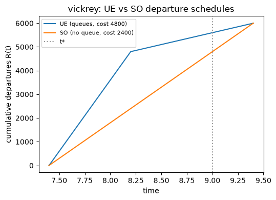
Visualize

tabench.viz is a road-network visualizer, and a single point-queue bottleneck has no network to draw — this notebook instead plots the two certified cumulative departure curves directly (a house departure-diagram, not tabench.viz): the SO’s straight-line uniform loading against the UE’s queue-building/dissipating kinks.

import matplotlib.pyplot as plt

fig, ax = plt.subplots(figsize=(5.5, 4.0))
ax.plot(ue.times, ue.cumulative, label=f"UE (queues, cost {m_ue['total_cost']:.0f})")
ax.plot(so.times, so.cumulative, label=f"SO (no queue, cost {m_so['total_cost']:.0f})")
ax.axvline(scenario.t_star, color="0.6", linestyle=":", label="t*")
ax.set_xlabel("time")
ax.set_ylabel("cumulative departures R(t)")
ax.set_title("vickrey: UE vs SO departure schedules")
ax.legend(fontsize=8)
fig.tight_layout()
display(fig)
plt.close(fig)

Takeaways & pointers

• Certified, not self-reported. Both schedules’ costs and gaps came from BottleneckEvaluator, reconstructed from the emitted R(t) alone; the solvers’ own r_early/t1/C* provenance was never trusted.

• PoA = 2 is exact, not a bound — the certified totals above land on it to three decimal places on this worked instance.

• Where next. the multi-route generalization vi-due (reduces to vickrey on one route with f=0); the lineage in the model compendium.