ltm — Yperman’s (2007) Link Transmission Model

What. ltm is the Newell-Daganzo cumulative-curve loading method as a LinkModel: sending reads Newell’s shifted UPSTREAM curve L/vf ahead (the point-queue look-ahead), and receiving adds a finite backward wave — storage freed by a downstream departure reappears at the upstream end L/w later. It is STATELESS beyond the base cumulative curves (no cells, _advance_state is a no-op): the whole link is evaluated by exact interpolation of piecewise-linear curves, not a grid of cell averages.

Why it is in the benchmark. It is ctm’s cumulative-curve twin — same sending/receiving interface, same physics, but no CFL = 1 cell-alignment requirement, only a wave-resolved grid dt <= min(L/vf, L/w). On any scenario where both are exact it must reproduce ctm’s boundary curves byte-for-byte; its concrete advantage is running on grids CTMLink rejects outright. See the model compendium (Yperman 2007) and docs/design/adr-016-ltm.md (P1).

Scope. This notebook loads the same built-in triangular_bottleneck_dynamic_scenario as ctm through LTMLink, certifies it, and cross-checks the two models’ cumulative curves. It also demonstrates LTM’s grid flexibility on a link CTMLink cannot load at all.

Canon. [yperman2007link], docs/REFERENCES.md / docs/references.bib.

How this notebook is graded

A notebook never claims a number it does not compute in that cell. Every scored quantity below is recomputed live by the P1 DNLEvaluator from the cumulative link curves the loader emitted, in the cell where it is claimed. LTM has no self-report to diff — like ctm, NetworkLoader.run() is a deterministic, one-shot forward simulation (README, Certified, not self-reported).

# Setup. `ltm` is a core DNL link model: a plain `pip install -e .` suffices —
# no optional extra, so no guard cell. The inline backend is Agg-based (headless
# CI renders into the notebook); NEVER matplotlib.use("Agg") in-kernel — it
# silently suppresses inline figure capture.
%matplotlib inline
import numpy as np

from tabench import (
    CTMLink,
    DNLEvaluator,
    DynamicDemand,
    DynamicScenario,
    LinkDynamics,
    LTMLink,
    NetworkLoader,
    TimeGrid,
    triangular_bottleneck_dynamic_scenario,
    viz,
)
from tabench.core.scenario import Network

The scenario

The same built-in triangular_bottleneck_dynamic_scenario ctm runs on (symmetric vf = w = 1, kappa = 4, capacities [2, 0.5], arrival rate 1.5) — both link models exact on this instance, so it is the fair cross-check anchor.

scenario = triangular_bottleneck_dynamic_scenario()
net = scenario.network
edges = scenario.grid.edges
print(f"scenario      : {scenario.name}")
print(f"content hash  : {scenario.content_hash()[:16]}…")
print(f"links         : {net.n_links}  (tail→head: "
      + ", ".join(f"{i}->{j}" for i, j in zip(net.init_node, net.term_node)) + ")")
print(f"grid          : dt={scenario.grid.dt}, n_steps={scenario.grid.n_steps}")
print("task          : deterministic DNL loading (feasibility + conservation + shock)")

scenario      : dnl-triangular-bottleneck
content hash  : d4148843c3292e42…
links         : 2  (tail→head: 1->3, 3->2)
grid          : dt=1.0, n_steps=12
task          : deterministic DNL loading (feasibility + conservation + shock)

Load the network

LTMLink needs only a finite jam density — no cell-alignment requirement — so the SAME NetworkLoader contract that ran ctm runs ltm unchanged.

out = NetworkLoader(scenario, LTMLink).run()
print(f"link model        : {LTMLink.__name__}")
print(f"emitted n_in[0]    : {np.round(out.n_in[0, ::4], 3)}  (every 4th edge)")
print(f"emitted n_out[0]   : {np.round(out.n_out[0, ::4], 3)}  (every 4th edge)")
print(f"storage at t={edges[-1]:.0f}      : {out.n_in[0, -1] - out.n_out[0, -1]:.3f}")

link model        : LTMLink
emitted n_in[0]    : [ 0.  6. 12. 18.]  (every 4th edge)
emitted n_out[0]   : [0. 0. 2. 4.]  (every 4th edge)
storage at t=12      : 14.000

Certify (P1) — feasibility, conservation, and byte-exact agreement with ctm

Both models are exact on this symmetric FD at CFL = 1, so LTM must reproduce CTM’s cumulative curves to machine precision — this is the distinctive LTM result, recomputed here by actually RUNNING ctm again in this cell (not quoting 01-ctm’s numbers) and diffing.

metrics = DNLEvaluator(scenario).evaluate(out)
print(f"dnl_feasible            : {metrics['dnl_feasible']:.0f}")
print(f"conservation_residual   : {metrics['conservation_residual']:.3e}")
print(f"storage_residual        : {metrics['storage_residual']:.3e}")
assert metrics["dnl_feasible"] == 1.0
assert metrics["conservation_residual"] <= 1e-9
assert metrics["storage_residual"] <= 1e-9

# The RH-shock boundary anchor, recomputed from the physical parameters exactly
# as in 01-ctm.ipynb (not quoted from it).
expected_n_in = 1.5 * edges
expected_n_out = np.maximum(0.0, 0.5 * (edges - 4.0))
np.testing.assert_allclose(out.n_in[0], expected_n_in, atol=1e-9)
np.testing.assert_allclose(out.n_out[0], expected_n_out, atol=1e-9)
print("boundary curves match the recomputed RH-shock anchor exactly (atol=1e-9)")

# DISTINCTIVE: byte-exact agreement with ctm, RE-RUN here (not quoted).
ctm_out = NetworkLoader(scenario, CTMLink).run()
np.testing.assert_array_equal(out.n_in, ctm_out.n_in)
np.testing.assert_array_equal(out.n_out, ctm_out.n_out)
print("ltm reproduces ctm's cumulative curves byte-for-byte "
      f"(max diff {np.abs(out.n_in - ctm_out.n_in).max():.1f})")

dnl_feasible            : 1
conservation_residual   : 0.000e+00
storage_residual        : 0.000e+00
boundary curves match the recomputed RH-shock anchor exactly (atol=1e-9)
ltm reproduces ctm's cumulative curves byte-for-byte (max diff 0.0)

LTM’s advantage: grids ctm cannot load

CTMLink requires a cell-aligned length L = n * vf * dt; LTMLink only needs dt <= min(L/vf, L/w) (wave-resolved). A single link with L=3, vf=2, dt=1 gives L/vf = 1.5 — not an integer, so CTMLink refuses it outright, while LTMLink free-flow-translates it exactly via the exact cumulative-curve interpolation (recomputed here, not quoted).

unaligned_net = Network(
    name="ltm-unaligned", n_nodes=2, n_zones=2, first_thru_node=1,
    init_node=np.array([1], dtype=np.int64), term_node=np.array([2], dtype=np.int64),
    capacity=np.ones(1), length=np.zeros(1), free_flow_time=np.ones(1),
    b=np.zeros(1), power=np.ones(1), toll=np.zeros(1), link_type=np.ones(1, dtype=np.int64),
)
rates = np.zeros((1, 2, 2))
rates[0, 0, 1] = 1.0
unaligned = DynamicScenario(
    name="ltm-unaligned", network=unaligned_net,
    dynamics=LinkDynamics(
        length=np.array([3.0]), free_speed=np.array([2.0]), wave_speed=np.array([1.0]),
        jam_density=np.array([3.0]), capacity=np.array([2.0]),
    ),
    demand=DynamicDemand(breakpoints=np.array([0.0, 4.0]), rates=rates),
    grid=TimeGrid(dt=1.0, n_steps=10),
)

try:
    NetworkLoader(unaligned, CTMLink).run()
    raise AssertionError("expected CTMLink to reject the unaligned length")
except ValueError as exc:
    print(f"CTMLink refuses this link: {exc}")

u_out = NetworkLoader(unaligned, LTMLink).run()
u_edges = unaligned.grid.edges
u_expected = np.minimum(np.maximum(u_edges - 1.5, 0.0), 4.0)  # free-flow lag L/vf = 1.5
np.testing.assert_allclose(u_out.n_out[0], u_expected, atol=1e-12)
u_metrics = DNLEvaluator(unaligned).evaluate(u_out)
assert u_metrics["dnl_feasible"] == 1.0
print("LTM loads the unaligned link exactly (L/vf = 1.5 lag) where CTM cannot")

CTMLink refuses this link: CTMLink needs a cell-aligned length L = n*vf*dt (CFL = 1): L=3.0, vf*dt=2.0 give 1.5 cells, not an integer >= 1
LTM loads the unaligned link exactly (L/vf = 1.5 lag) where CTM cannot

Visualize

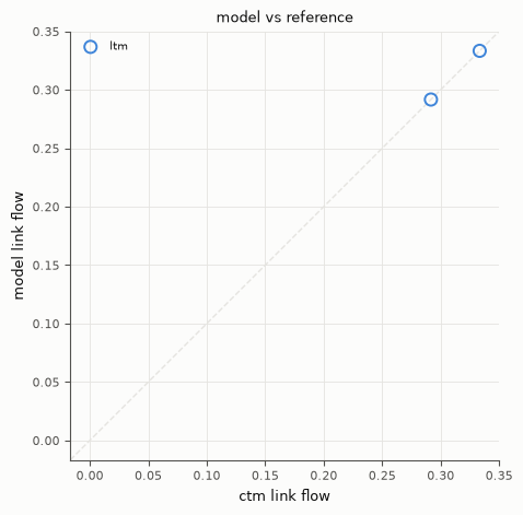
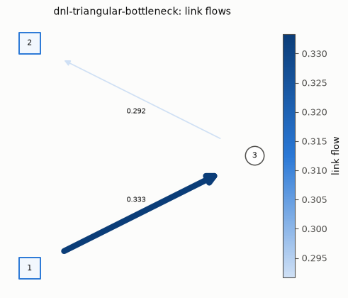
Both figures come from tabench.viz, the house visualizer. Left/top: the certified bottleneck network coloured by each link’s time-averaged flow. Right/bottom: LTM’s average flow against CTM’s — every point sits on y = x (the byte-exact agreement certified above).

T = float(edges[-1])
ltm_avg = out.n_out[:, -1] / T
ctm_avg = ctm_out.n_out[:, -1] / T

display(viz.plot_network_flows(net, ltm_avg))
display(viz.plot_flow_scatter(("ctm", ctm_avg), {"ltm": ltm_avg}))

Takeaways & pointers

• Certified, not self-reported. DNL link models have nothing to self-report — the boundary curves above ARE the emitted output, recertified from scratch by DNLEvaluator.

• Exact where both are exact, flexible where ctm is not. LTM’s cumulative- curve evaluation carries no interior discretisation, so it needs no CFL = 1 cell alignment — the concrete win demonstrated above.

• Where next. the cell-based twin ctm; the smooth non-triangular FD godunov (built on the same ctm cell update); merges/diverges node-model; the lineage in the model compendium.