dtd-cumlog — Li, Wang & Nie’s (2024) cumulative-logit day-to-day dynamics

Every logit-choice day-to-day model shipped so far rests at stochastic user equilibrium (dtd-horowitz, dtd-stochastic, dtd-swap-sue), and every model whose limit is deterministic Wardrop UE uses a perfectly rational adjustment direction (dtd-swap, dtd-friesz, dtd-link). CumLog (li2024wardrop) fills the empty cell: a boundedly-rational logit choice — travelers put positive probability on acceptable suboptimal routes every day — whose global limit is nonetheless exact Wardrop UE at a finite exploitation parameter r.

The trick is one line. Travelers carry a per-OD route-valuation vector s, choose by the logit map p = softmax(-r s), and accumulate the experienced route cost s <- s + eta_t c(p) (Eq. 6) rather than average it s <- (1-eta_t) s + eta_t c(p) (Eq. 4, the classical scheme whose limit is SUE). This notebook certifies both halves of that contrast (Remark 3) on identical machinery.

How this notebook is graded

A notebook never claims a number it does not compute in that cell. Every scored quantity below is recomputed live by the P1 Evaluator from the flows the model emitted, in the cell where it is claimed. Model self-reports (the per-day relative gap) are shown only as provenance and diffed against the certificate, exactly as the harness treats them (README, Certified, not self-reported). Analytic anchors (the exact Braess UE, the binary-logit SUE split) are recomputed in-cell, never quoted.

# Setup. `dtd-cumlog` is a core day-to-day model: a plain `pip install -e .` suffices —
# no optional extra, so no guard cell. The inline backend is Agg-based (headless CI
# renders into the notebook); NEVER matplotlib.use("Agg") in-kernel — it silently
# suppresses inline figure capture.
%matplotlib inline
import numpy as np
from scipy.optimize import brentq

from tabench import (
    Budget,
    CumLogDTDModel,
    Evaluator,
    RngBundle,
    Trace,
    braess_scenario,
    two_route_scenario,
    viz,
)

The scenario

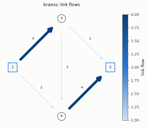
The classic Braess network (unique UE link flows [4, 2, 2, 2, 4], common route time 92) for the exact-UE limit, and the two-route anchor — taken as a deterministic UE task (sue_theta=None) so the certificate is the standard Wardrop relative gap — for the accumulation-vs-averaging headline, where its analytic limits are hand-checkable.

braess = braess_scenario()
net = braess.network
anchor = two_route_scenario(sue_theta=None)  # deterministic UE certificate
print(f"braess       : {net.n_links} links, demand {braess.demand.total:g}")
# This model adds NO scenario field, so the golden Braess content hash is
# byte-identical to every other row's (the witness for the takeaways claim below).
print(f"content hash : {braess.content_hash()[:16]}…")
print(f"two-route    : {anchor.network.n_links} links, demand {anchor.demand.total:g}")

braess       : 5 links, demand 6
content hash : cf00f411cdccec88…
two-route    : 4 links, demand 4

Run the cumulative-logit process

Default factors: exploitation r = 1, the harmonic schedule eta_t = 1/(t+1) (which converges to WE for any r, Theorem 1(i)), accumulation on. One batched Dijkstra per day grows the working route set and supplies SPTT for the gap.

run = Trace()
model = CumLogDTDModel(r=1.0)  # harmonic default, accumulate=True
model.solve(braess, Budget(iterations=5000, target_relative_gap=1e-7), RngBundle(0), run)
final = run.final
print(f"model          : {model.name}")
print(f"days simulated : {final.coords.iterations}  ({final.coords.sp_calls} shortest-path calls)")
print(f"emitted flows  : {np.round(final.link_flows, 6)}")
print(f"self-reported relative gap : {final.self_report['relative_gap']:.3e}  (provenance only)")

model          : dtd-cumlog
days simulated : 27  (28 shortest-path calls)
emitted flows  : [4.000001 1.999999 2.000003 1.999999 4.000001]
self-reported relative gap : 6.913e-08  (provenance only)

Certify (P1) — exact deterministic Wardrop UE

The rest point is Wardrop UE, so the scored quantity is the standard UE relative gap the harness recomputes from the emitted link flows — no new certificate, no new scenario field. A finite-r logit choice, yet the limit is the exact UE (not the SUE an averaged-cost logit would give).

metrics = Evaluator(braess).evaluate(final.link_flows)
print(f"certified UE relative gap : {metrics['relative_gap']:.3e}")
print(f"feasible                  : {metrics['feasible']:.0f}")
assert metrics["feasible"] == 1.0
assert metrics["relative_gap"] < 1e-6

# The exact analytic Braess UE (2 units on each of the three routes).
ue_flows = np.array([4.0, 2.0, 2.0, 2.0, 4.0])
assert np.allclose(final.link_flows, ue_flows, atol=1e-3)
print(f"emitted flows == exact Braess UE {ue_flows.tolist()}")

# Honesty (P1): the model self-reports the SAME relative gap the harness recomputes.
assert np.isclose(final.self_report["relative_gap"], metrics["relative_gap"], rtol=1e-9, atol=1e-12)
print("self-report == certificate (P1)")

certified UE relative gap : 6.913e-08
feasible                  : 1
emitted flows == exact Braess UE [4.0, 2.0, 2.0, 2.0, 4.0]
self-report == certificate (P1)

The headline — accumulation vs averaging (Remark 3)

The paper’s central claim as an executable fact on one instance, identical machinery, the same r = 1: the one-line difference between Eq. 6 (accumulate) and Eq. 4 (average) is the difference between converging to exact Wardrop UE and converging to the logit SUE. accumulate=False is a comparison knob for this contrast — never a shipped SUE mode (dtd-horowitz remains the benchmark’s logit-SUE day-to-day row).

ev = Evaluator(anchor)

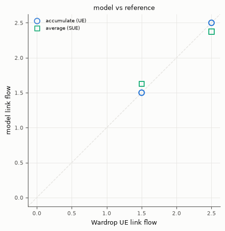
# Eq. 6 (accumulate) -> exact deterministic Wardrop UE: f_A -> 2.5.
acc = Trace()
CumLogDTDModel(r=1.0, accumulate=True).solve(
    anchor, Budget(iterations=6000, target_relative_gap=1e-7), RngBundle(0), acc
)
m_acc = ev.evaluate(acc.final.link_flows)
print(f"accumulate (Eq. 6) : f_A = {acc.final.link_flows[0]:.6f}   UE gap = {m_acc['relative_gap']:.2e}")
assert m_acc["feasible"] == 1.0 and m_acc["relative_gap"] < 1e-6

# Eq. 4 (average) -> the logit SUE at dispersion r: the binary-logit split, recomputed in-cell.
avg = Trace()
CumLogDTDModel(r=1.0, accumulate=False).solve(anchor, Budget(iterations=4000), RngBundle(0), avg)
m_avg = ev.evaluate(avg.final.link_flows)
def _sue_resid(f_a):
    c_a, c_b = 2.0 + f_a, 1.5 + 2.0 * (4.0 - f_a)
    return f_a - 4.0 / (1.0 + np.exp(1.0 * (c_a - c_b)))  # dispersion r = 1
f_a_sue = brentq(_sue_resid, 0.0, 4.0, xtol=1e-12)
print(f"average    (Eq. 4) : f_A = {avg.final.link_flows[0]:.6f}   UE gap = {m_avg['relative_gap']:.3f}   (analytic SUE {f_a_sue:.6f})")
assert np.isclose(avg.final.link_flows[0], f_a_sue, atol=1e-3)  # matches the analytic SUE
assert m_avg["relative_gap"] > 0.01  # NOT deterministic UE

# One line changed; a categorically different limit.
assert abs(acc.final.link_flows[0] - avg.final.link_flows[0]) > 0.1
print(f"\nsame machinery, same r=1: accumulate -> exact UE (2.5), average -> logit SUE ({f_a_sue:.4f})")

accumulate (Eq. 6) : f_A = 2.500000   UE gap = 9.98e-08
average    (Eq. 4) : f_A = 2.373888   UE gap = 0.034   (analytic SUE 2.373888)


same machinery, same r=1: accumulate -> exact UE (2.5), average -> logit SUE (2.3739)

Visualize

# Certified terminal flows on the Braess network (house style via tabench.viz).
display(viz.plot_network_flows(net, final.link_flows))

# The headline, on the two-route anchor: accumulation lands on the Wardrop UE (on the
# diagonal), the one-line-different averaging variant lands on the logit SUE (off it).
ue_two_route = np.array([2.5, 2.5, 1.5, 1.5])
display(viz.plot_flow_scatter(
    ("Wardrop UE", ue_two_route),
    {"accumulate (UE)": acc.final.link_flows, "average (SUE)": avg.final.link_flows},
))

Takeaways & pointers

• Certified, not self-reported. The UE gap came from Evaluator — the standard Wardrop relative gap, no new certificate and no new scenario field (the golden Braess hash is byte-identical).

• One line, two limits. Accumulating the experienced cost (Eq. 6) reaches exact Wardrop UE at a finite r; averaging it (Eq. 4) reaches the logit SUE — the same machinery, the same r, a categorically different limit (Remark 3).

• Bounded rationality, two ways. CumLog’s is process-level (imperfect choices along the path, WE preserved); br-ue’s is concept-level (an indifference band relaxes the equilibrium itself). See ADR-038 vs ADR-008.

• Where next. the SUE sibling that averages dtd-horowitz; the route-swap UE process dtd-swap; the lineage in the model compendium.