od-congested — Yang, Sasaki, Iida & Asakura’s (1992) bilevel OD estimation

What. od-congested (Yang1992Estimator, T2, ADR-002) is a bilevel program with a SINGLE trade-off dial theta (unlike gls’s per-cell covariance weighting): min_g theta*(g-g_pr)'(g-g_pr) + (1-theta)*(p g - c)'(p g - c), solved as an inner MSA assignment feeding an outer QP with UNIFORM weighting on every cell/residual. It is the congested-network extension of the classical bilevel OD estimation literature (Yang 1995’s sensitivity-analysis lineage traces back to this 1992 formulation).

Why it is in the benchmark. theta gives an exact, hand-verifiable prior<->count spectrum (theta->1 = pure prior, theta->0 = pure count fit) that gls’s per-cell covariances do not expose as a single scalar — and because Yang’s uniform weighting is mathematically DIFFERENT from gls’s per-cell variance weighting, the two estimators allocate an under-identified fit differently even though yang_solve IS gls_solve at specific scalar variances. See the model compendium (Yang, Sasaki, Iida & Asakura 1992) and docs/design/adr-002-t2-estimation-certificate.md (P1).

Scope. The scalar closed form and its exact gls_solve equivalence, the theta prior<->count spectrum, the uniform-vs-covariance weighting divergence, and the congested-network theta->0 recovery on Braess.

Canon. [yang1992estimation], docs/REFERENCES.md / docs/references.bib.

How this notebook is graded

A notebook never claims a number it does not compute in that cell. Every scored quantity below is recomputed live — the closed forms are recomputed algebraically in-cell (no trusted digits), and the Braess recovery is recomputed by the P1 ODCertifier from the emitted OD matrix against the harness’s own pinned BFW assignment, never from od-congested’s self-report (README, Certified, not self-reported).

# Setup. `od-congested` is a core estimator: a plain `pip install -e .`
# suffices — no optional extra, so no guard cell. The inline backend is
# Agg-based (headless CI renders into the notebook); NEVER
# matplotlib.use("Agg") in-kernel — it silently suppresses inline capture.
%matplotlib inline
import numpy as np

from tabench import (
    Budget,
    Demand,
    ODCertifier,
    RngBundle,
    Trace,
    braess_scenario,
    two_route_scenario,
    viz,
)
from tabench.core.rng import SOURCE_OBSERVATION
from tabench.estimation import ODTrace, Yang1992Estimator, gls_solve, yang_solve
from tabench.estimation.base import EstimationTask
from tabench.models.frank_wolfe import BiconjugateFrankWolfeModel
from tabench.observe.levels import LinkCounts

BRAESS_TRUTH = np.array([4.0, 2.0, 2.0, 2.0, 4.0])  # UE(D=6), recomputed below
TWOROUTE_TRUTH = np.array([2.5, 2.5, 1.5, 1.5])  # UE(D=4), recomputed below

# Analytic anchors recomputed, never quoted: pin both by an independent
# high-precision BFW solve before EITHER constant is used as a data-generating
# truth anywhere below.
def _pinned_ue(scenario):
    trace = Trace()
    BiconjugateFrankWolfeModel().solve(
        scenario, Budget(iterations=5000, target_relative_gap=1e-10), RngBundle(0), trace
    )
    return trace.final.link_flows

np.testing.assert_allclose(_pinned_ue(braess_scenario(6.0)), BRAESS_TRUTH, atol=1e-6)
np.testing.assert_allclose(_pinned_ue(two_route_scenario(sue_theta=None)), TWOROUTE_TRUTH, atol=1e-6)

The closed form: theta-weighted, and exactly a gls special case

Single pair, single sensor: g* = (theta*g_pr + (1-theta)*p*c) / (theta + (1-theta)*p^2). At the scalar variances W=1/theta, V=1/(1-theta), this is LITERALLY gls_solve — the exact sense in which od-congested is the deterministic-tradeoff special case of generalized least squares.

p, c, g_pr = 0.625, 2.5, 3.0
for theta in (0.2, 0.5, 0.8):
    expected = (theta * g_pr + (1 - theta) * p * c) / (theta + (1 - theta) * p * p)
    got = yang_solve(np.array([[p]]), np.array([c]), np.array([g_pr]), theta)
    via_gls = gls_solve(
        np.array([[p]]), np.array([c]), np.array([g_pr]),
        np.array([1.0 / theta]), np.array([1.0 / (1.0 - theta)]),
    )
    print(f"theta={theta}: yang_solve={got[0]:.6f}  closed form={expected:.6f}  via gls_solve={via_gls[0]:.6f}")
    assert np.isclose(got[0], expected, atol=1e-10)
    assert np.isclose(got[0], via_gls[0], atol=1e-9)

theta=0.2: yang_solve=3.609756  closed form=3.609756  via gls_solve=3.609756
theta=0.5: yang_solve=3.280899  closed form=3.280899  via gls_solve=3.280899
theta=0.8: yang_solve=3.088968  closed form=3.088968  via gls_solve=3.088968

The distinctive knob: theta spans the whole prior<->count spectrum

theta -> 1 recovers the prior exactly; theta -> 0 fits the count exactly (c/p) — the single scalar dial this estimator is named for.

p2, c2, g_pr2 = 0.5, 3.0, 1.0
near_prior = yang_solve(np.array([[p2]]), np.array([c2]), np.array([g_pr2]), 1 - 1e-8)[0]
near_count = yang_solve(np.array([[p2]]), np.array([c2]), np.array([g_pr2]), 1e-8)[0]
print(f"theta->1 (near_prior) : {near_prior:.6f}  (prior: {g_pr2})")
print(f"theta->0 (near_count) : {near_count:.6f}  (c/p: {c2 / p2:.6f})")
assert np.isclose(near_prior, g_pr2, atol=1e-4)
assert np.isclose(near_count, c2 / p2, atol=1e-4)

theta->1 (near_prior) : 1.000000  (prior: 1.0)
theta->0 (near_count) : 6.000000  (c/p: 6.000000)

Not a gls rename: uniform vs per-cell covariance weighting

Given a count the prior does NOT already satisfy, gls loads most of the adjustment onto the more-uncertain (large-prior) cell (per-cell covariance W), while od-congested’s uniform theta splits the residual evenly across cells — so the two allocate the fit differently, not just by a constant rescaling.

p_obs = np.array([[1.0, 1.0]])  # one sensor sees both pairs
c3 = np.array([14.0])            # prior sum (2+8=10) does NOT match it
g_pr3 = np.array([2.0, 8.0])    # priors of very different magnitude
yang = yang_solve(p_obs, c3, g_pr3, 0.5)          # uniform weighting: near-even split
w_var = (0.5 * g_pr3) ** 2 + 1e-6                  # gls: large-prior cell far more uncertain
gls = gls_solve(p_obs, c3, g_pr3, w_var, np.array([1.0]))
print(f"yang_solve (uniform)         : {np.round(yang, 4)}")
print(f"gls_solve (per-cell weighted): {np.round(gls, 4)}")
print(f"max |yang - gls|             : {np.abs(yang - gls).max():.4f}")
assert np.abs(yang - gls).max() > 0.5
# gls moves the uncertain (large-prior) cell much more than yang's uniform split.
assert (gls[1] - g_pr3[1]) > (yang[1] - g_pr3[1]) + 0.5

yang_solve (uniform)         : [3.3333 9.3333]
gls_solve (per-cell weighted): [ 2.2222 11.5556]
max |yang - gls|             : 2.2222

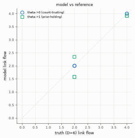
Congested-network recovery: theta->0 trusts the counts

On both the convex two-route corridor (D=4) and the Braess network (D=6, from the global-basin prior D=5.5 — see spiess for the SPURIOUS-basin caveat this same network has), the bilevel outer fixed point recovers the equilibrium-consistent truth as theta -> 0 (count-trusting); at theta -> 1 it instead holds at the prior. braess_scenario(6.0) is frozen and content-hashed (P2).

def _single_pair_prior(d):
    m = np.zeros((2, 2))
    m[0, 1] = d
    return m


def _task(scenario, truth, sensors, prior_matrix):
    ds = LinkCounts(np.asarray(sensors), 1, "none").observe(
        scenario, truth, RngBundle(0).generator(SOURCE_OBSERVATION)
    )
    return EstimationTask(
        name="t", network=scenario.network, prior=Demand(np.asarray(prior_matrix, dtype=np.float64)),
        dataset=ds, identifiability={}, scenario_hash=scenario.content_hash(), seed=0,
    )


budget = Budget(sp_calls=10**9, iterations=200)
for scenario_fn, truth, prior_d, target, label in (
    (lambda: two_route_scenario(sue_theta=None), TWOROUTE_TRUTH, 3.0, 4.0, "two-route"),
    (lambda: braess_scenario(6.0), BRAESS_TRUTH, 5.5, 6.0, "braess"),
):
    sc = scenario_fn()
    task = _task(sc, truth, np.arange(len(truth)), _single_pair_prior(prior_d))
    trace_count = ODTrace()
    Yang1992Estimator(k_inner=120, outer_iters=80, theta=1e-3).estimate(
        task, budget, RngBundle(0), trace_count
    )
    trace_prior = ODTrace()
    Yang1992Estimator(k_inner=120, outer_iters=30, theta=1 - 1e-6).estimate(
        task, budget, RngBundle(0), trace_prior
    )
    d_count, d_prior = trace_count.final.od_matrix[0, 1], trace_prior.final.od_matrix[0, 1]
    print(f"{label}: theta->0 = {d_count:.4f} (target {target}); "
          f"theta->1 = {d_prior:.4f} (prior {prior_d})")
    assert abs(d_count - target) < 1e-2
    assert abs(d_prior - prior_d) < 1e-2

sc_final = braess_scenario(6.0)
print(f"content hash  : {sc_final.content_hash()[:16]}…")
certifier = ODCertifier(
    sc_final, np.arange(5), np.array([], dtype=np.int64),
    BRAESS_TRUTH[None, :], BRAESS_TRUTH[[]][None, :], BRAESS_TRUTH,
    {"linear_identifiable": True},
)
metrics = certifier.certify(trace_count.final.od_matrix)
print(f"certified od_rmse (Braess, theta->0) : {metrics['od_rmse']:.4e}")
assert metrics["od_feasible"] == 1.0
assert metrics["od_rmse"] < 1e-2

two-route: theta->0 = 3.9991 (target 4.0); theta->1 = 3.0000 (prior 3.0)
braess: theta->0 = 5.9996 (target 6.0); theta->1 = 5.5000 (prior 5.5)
content hash  : cf00f411cdccec88…
certified od_rmse (Braess, theta->0) : 2.8932e-04

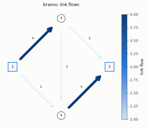
Visualize

tabench.viz draws the road Network’s link flows for the count-trusting (theta->0) recovery vs the prior-holding (theta->1) estimate on Braess, both re-assigned from the certified OD matrices above.

from tabench import Scenario
count_trace = Trace()
BiconjugateFrankWolfeModel().solve(
    Scenario("count-trusting", sc_final.network, Demand(trace_count.final.od_matrix), family=sc_final.family),
    Budget(iterations=5000, target_relative_gap=1e-10), RngBundle(0), count_trace,
)
prior_hold_trace = Trace()
BiconjugateFrankWolfeModel().solve(
    Scenario("prior-holding", sc_final.network, Demand(trace_prior.final.od_matrix), family=sc_final.family),
    Budget(iterations=5000, target_relative_gap=1e-10), RngBundle(0), prior_hold_trace,
)
display(viz.plot_network_flows(sc_final.network, BRAESS_TRUTH))
display(viz.plot_flow_scatter(
    ("truth (D=6)", BRAESS_TRUTH),
    {"theta->0 (count-trusting)": count_trace.final.link_flows,
     "theta->1 (prior-holding)": prior_hold_trace.final.link_flows},
))

Takeaways & pointers

• Certified, not self-reported. The Braess od_rmse above came from ODCertifier’s own re-assignment of the emitted OD matrix, never from od-congested’s inner-MSA proportions.

• A single scalar dial, exactly a gls special case at fixed variances — but not a rename at the estimator level. Uniform-vs-per-cell weighting is verified above to allocate an under-identified fit differently.

• Where next. the per-cell-covariance sibling gls; the count-only end of the spectrum spiess; the lineage in the model compendium.